pyViewFactor v1.1.0 — SA-30 kernel & BVH acceleration
A year after the last significant update to pyViewFactor , version 1.1.0 brings a significant rework of the integration algorithms. On the agenda: a semi-analytic integration kernel that eliminates numerical bias on closed meshes, and a hierarchical bounding volume structure to accelerate obstruction tests — all JIT-compiled with Numba for a measured ~33× speedup on a reference urban case.
Background: the problem
The view factor $F_{i \to j}$ quantifies the fraction of radiation emitted by surface $i$ that reaches surface $j$:
$$ F_{i \to j} = \frac{1}{A_i} \iint_{A_i} \iint_{A_j} \frac{\cos\theta_i \cos\theta_j}{\pi r^2} dA_i dA_j $$For arbitrary planar polygons, Mazumder & Ravishankar (2012) show that a double application of Green’s theorem reduces this surface integral to a contour integral:
$$ A_i F_{i \to j} = \frac{1}{2\pi} \oint_{\partial A_i} \oint_{\partial A_j} \ln(r_{kl}) d\mathbf{k} \cdot d\mathbf{l} $$Discretising the contours into directed edges gives a sum over all edge pairs $(k, l)$:
$$ A_i F_{i \to j} = \frac{1}{4\pi} \sum_{k} \sum_{l} (\mathbf{e}_{k} \cdot \mathbf{e}_{l}) \int_0^1 \int_0^1 \ln r_{kl}^{2}(t, s) \, dt \, ds $$where $r^2_{kl}(t,s)$ is a degree-2 polynomial in $t$ and $s$. This is the form on which all library kernels operate.
The v1.0 kernel problem
In v1.0.3, the matrix computation started with a pair classification step: faces sharing a vertex or edge (touching) were separated from disjoint pairs. Each group was then handled differently:
- Touching pairs →
dblquad+ epsilon shift: face $j$ was slightly displaced in the centroid-to-centroid direction before integration, to push the $\ln(r^2)$ singularity away. Epsilon was a tunable parameter — too small and the singularity remained problematic; too large and the geometry was distorted enough to bias the result. The integral itself was then evaluated byscipy.integrate.dblquad(adaptive quadrature over both levels). - Disjoint pairs →
GL-30×30: 30-point Gauss–Legendre rule applied to each of the two integrals independently, no shift needed.
The outcome: on a closed mesh, the row sums of a face are systematically underestimated by about 0.16% — a structural bias tied to the epsilon shift, impossible to eliminate without changing the approach.
The v1.1.0 kernel solves this at the root.
Accuracy and speed: the Pareto chart
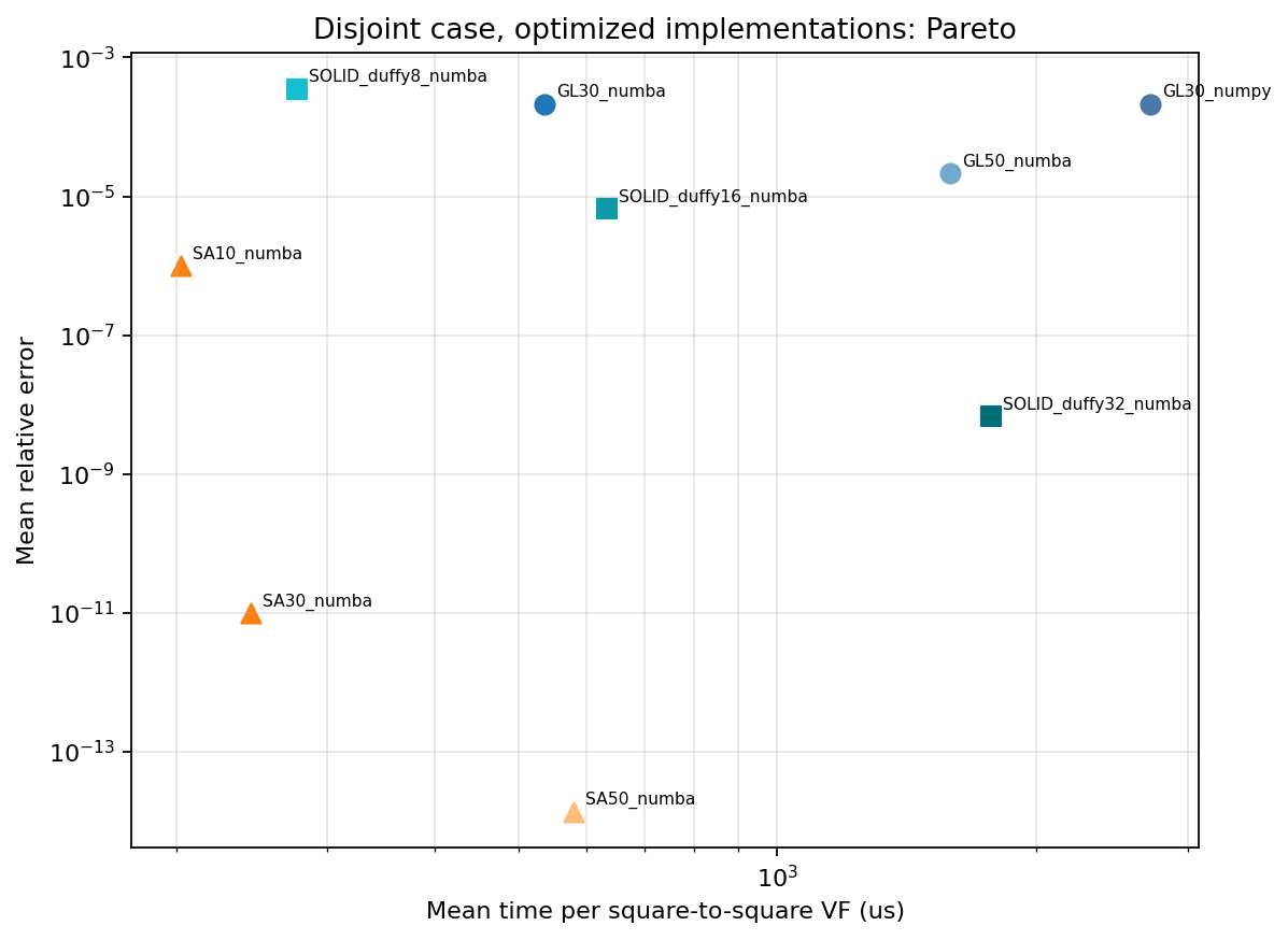
Accuracy vs. computation time per face pair (disjoint case). Bottom-left = optimal. The SA-30 kernel (orange triangles) clearly dominates GL-30 (blue circles, v1.0 kernel): relative error ~10⁻¹¹ vs ~10⁻⁴, at comparable speed.
The SA-30 kernel: closed-form inner integral
The SA-30 kernel (v1.1.0) evaluates the inner integral exactly, for each outer quadrature point. The integral to solve takes the form:
$$ I(x) = \int_0^1 \ln(A y^2 + B y + C) \, dy $$where $A$, $B$, $C$ are functions of the outer quadrature point $x$ and the edge pair. The discriminant $\Delta = 4AC - B^2$ determines the branch:
| Case | Condition | Closed form |
|---|---|---|
| Disjoint pair | $\Delta > 0$ | Arc-tangent formula |
| Tangent / coplanar pair | $\Delta \leq 0$ | Real-root decomposition |
The $\Delta \leq 0$ case is precisely that of adjacent or coplanar faces — handled exactly, without epsilon shift, without bias. Both directions $F(i \to j)$ and $F(j \to i)$ are computed independently (no reciprocity fill), which brings an additional precision benefit on closed meshes.
BVH acceleration for obstruction tests
For each face pair $(i, j)$, we need to check whether the centroid-to-centroid segment is blocked by a triangle of the obstacle mesh. In v1.0, a flat AABB pre-filter (combined bounding box of the two faces) already eliminated obviously out-of-range triangles — but the remaining candidates were then tested sequentially, one by one.
The idea: a hierarchy of bounding boxes (AABB)
A Bounding Volume Hierarchy (BVH) organises the obstacle triangles into a binary tree of axis-aligned bounding boxes (AABBs). Each tree node is an AABB containing all triangles in its subtree.
Construction (once, at preprocessing time):
- Compute the AABB of the current set of triangles.
- Split along the longest axis, at the median centroid.
- Recurse until each leaf contains a single triangle.
Traversal for a ray:
- Test the ray against the root node’s AABB (slab test: 6 comparisons).
- Miss → prune the entire subtree, zero triangles tested.
- Hit → recurse into both children.
- At a leaf → Möller–Trumbore test on the triangle.
Each tree level eliminates roughly half the remaining candidates: cost O(log N_tri) per ray instead of O(N_tri).
The tree is stored as five flat numpy arrays (node_mins, node_maxs, node_left, node_right, node_tri) — no pointers, no Python objects — for Numba-compatible traversal.
Results on the reference case
Urban mesh of 382 faces, 72,771 candidate pairs, full self-obstruction:
| Version | Integrator | Obstruction | Time | Speedup |
|---|---|---|---|---|
| ≤ v1.0 | GL-30 + dblquad | Linear scan O(N) | reference | 1× |
| v1.1.0 | SA-30 | BVH O(log N) + Numba prange | ~33× faster | 33× |
Both effects compound:
- BVH: reduces obstruction cost from O(N_tri) to O(log N_tri) per ray
- Numba
prange: parallelises both obstruction and integration over all pairs
New documentation: migration to MkDocs
Version 1.1.0 also brings a fully rewritten documentation. The auto-generation via pdoc has been replaced by MkDocs + mkdocstrings, with the Material theme.
The documentation is structured into four sections:
- Theory: derivation of the double integral, SA-30 semi-analytic kernel, BVH obstruction engine,
- Implementation: pipeline architecture, visibility & obstruction semantics, performance guide,
- Examples: from a single face pair to full urban scene analysis,
- API reference: auto-generated from NumPy-format docstrings.
Available at: arep-dev.gitlab.io/pyViewFactor
Installation
Numba is optional but strongly recommended. Without it, all kernels fall back to sequential pure Python with identical results.