 L'hypercube
UrbIrrad
UrbIrrad is an open-source Python tool for calculating solar irradiance on a sensor mesh. It prepares the scene, calls Radiance through PyRadiance, and packages the results in HDF5. It supports building and urban studies indoors, outdoors and in semi-open spaces.

The aim is to make solar calculations with Radiance more accessible, without having to assemble its command pipeline yourself. Provide geometry and weather data, define materials, sensors and dates in YAML, then run the calculation from your terminal. Install the library with python -m pip install urbirrad.
The simplest calculation gives direct sunlight received on a plane, accounting for shadows and transmission through glazing. You can then add sky-diffuse irradiance and diffuse reflections of direct sunlight, or calculate exposure in six directions. A separate geometric mode also provides potential sunshine hours.
Results are stored in HDF5, with an XDMF companion for exploration in ParaView. The tool handles shortwave solar radiation only: six-direction outputs can inform comfort studies, but UrbIrrad calculates neither longwave radiation nor complete mean radiant temperature. The full documentation describes settings and limitations for each option.
Required inputs
A case combines an EPW weather file, scene surfaces and a sensor mesh. A YAML file defines solar properties: reflectance for opaque surfaces, transmittance for glazing, receiving-plane orientation, dates and calculation components.
STL, VTP, VTK, OBJ and PLY are supported. Meshes must already be triangulated: there is no automatic repair or CAD import. Coordinates use X East, Y North, Z Up, in metres. Optical properties come from YAML, not file colours or textures.
Each sensor-mesh triangle provides a calculation point at its centre, with a configurable offset to avoid placing it exactly on a surface. In plane mode, a common normal defines all receiving-plane orientations; it is not inferred from triangle normals.
Three distinct components
| Component | Meaning | ParaView field |
|---|---|---|
| Direct | Sunlight received on the plane, with shadows and glazing transmission, without surface reflections | solar_direct |
| Diffuse | Sky contribution, with obstruction, transmission and permitted diffuse reflections | solar_diffuse |
| Reflected direct | Sunlight contributions involving at least one diffuse surface reflection | solar_direct_reflected |
Results are incident irradiances in W/m², not simply the weather file’s DNI or DHI. Grazing radiation contributes less than perpendicular radiation, and radiation arriving from behind the receiving plane does not contribute.
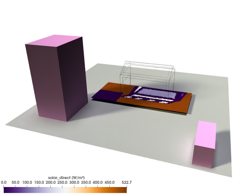
Direct: sunlight is evaluated at its hourly positions, including shadows and transmission through glazing.
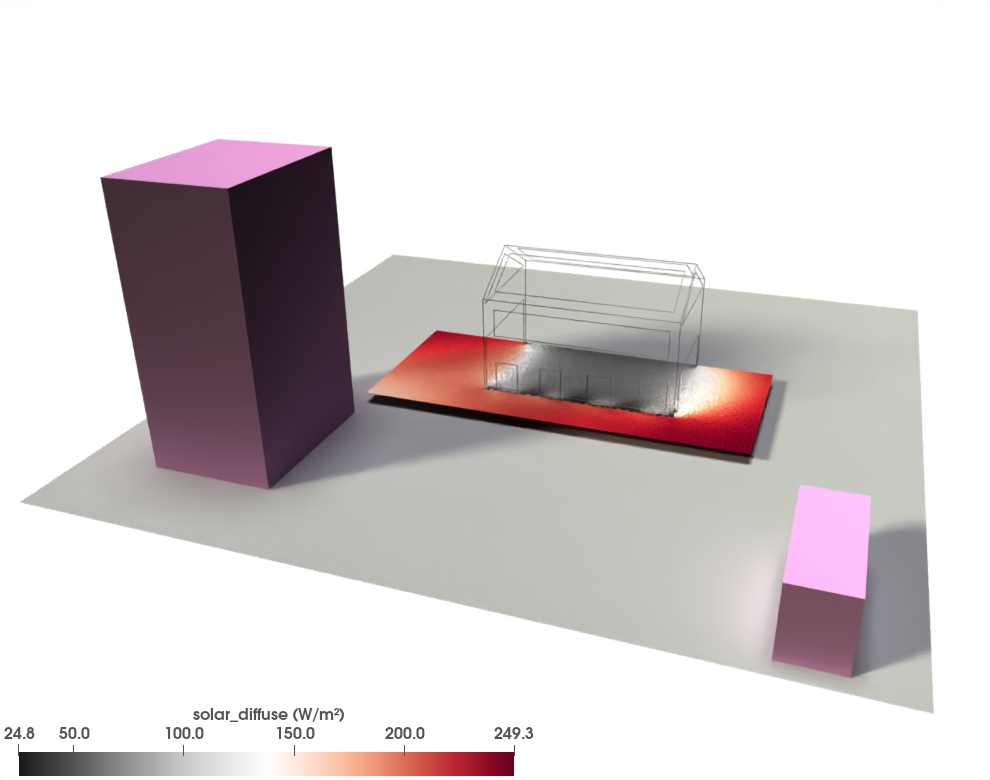
Diffuse: the sky is an extended source. Access depends on obstructions, openings and permitted reflection paths.
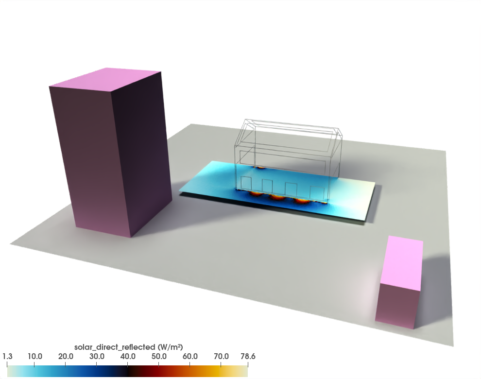
Reflected direct: an additional contribution driven by sunlight and scene surfaces. These figures use independent colour scales; compare the legends in W/m², not colours alone.
The diffuse component does not contain sun-driven reflections. These are calculated separately. Reflected direct is a sky-patch-based approximation; it excludes purely specular paths, such as sunlight reflected only by glass or a mirror.
Why use matrices
Radiance follows radiation paths from receivers towards sources. Integrating diffuse irradiance on a plane requires sampling a hemisphere and secondary paths: it is not just a shadow test.
For fixed geometry and materials, the scene’s response to different sky regions can be calculated once. UrbIrrad separates that geometric response from sky intensity, which changes with the weather:
$$ \mathbf{E} = \mathbf{C}\,\mathbf{S} $$Matrix C connects receiving planes to sky and ground patches; matrix S contains their intensities at each weather interval. Their product provides irradiances for every interval. This is a schematic expression: Radiance matrices carry three channels, subsequently reduced to scalar irradiance.
The main Radiance programs have distinct roles:
oconvcompiles an octree to accelerate ray/surface intersections.gendaymtxcreates weather-dependent skies and solar sources from the EPW.rfluxmtxcalculates transfer matrices through the scene.rcontribseparates source contributions, particularly for the direct calculation.dctimestepapplies sky matrices to coefficients without retracing geometry.
This avoids launching a complete scene calculation for every diffuse-weather interval. Loops, ray sampling, matrix multiplication and output writing still require work.
Direct uses a different approach: sources at the intervals’ solar positions are processed in a batch. It uses neither the sky-patch approximation nor dctimestep. For reflected direct, two traces use identical hemisphere rays with and without diffuse bounces; subtracting them isolates the reflected contribution and avoids counting direct sunlight twice.
Accuracy and runtime
Our trials show the following pattern:
| Calculation | Observed first-run cost |
|---|---|
| Direct | Very fast |
| Sky diffuse | Quite reasonable for the scenes tested |
| Reflected direct | Substantially longer; sampling reflected paths often dominates total runtime |
This is not a universal benchmark. Sensor count, six orientations instead of one, geometry, ray count, reflection depth and hardware all affect cost. --nproc parallelizes ray tracing, but doubling workers does not guarantee halving runtime. The terminal reports progress and stage timings.
Diffuse and reflected-direct coefficients are cached. Another period or weather file can reuse them when geometry, materials, sensors and numerical settings remain compatible. The cache does not remove direct computation, sky generation, matrix multiplication or output writing.
MF=1 represents the sky with 145 patches plus ground; MF=2 uses 577 sky patches plus ground. Finer resolution improves angular discretization at additional cost; it does not change the direct calculation’s solar positions.
The initial diffuse setting is ambient_bounces: 3. Receiving-plane integration consumes one Radiance ambient level, leaving up to two physical diffuse surface reflections. Reflected direct has separate settings. Example values do not replace scene-specific convergence checks.
Installation and execution
In a Python 3.12 or newer environment:
PyRadiance supplies the required Radiance executables on Windows. Example data are not included in the package; obtain them from the repository:
The default example calculates direct irradiance only. Separate YAML files progressively add diffuse sky, six directions and reflected direct. In a copied and adapted case, this configuration excerpt selects July and all three components:
Dates are inclusive and data paths are relative to the YAML file. This excerpt supplements an existing case; it does not replace weather, geometry and material definitions.
Six directions and sunshine hours
six_directions mode calculates six hemispherical irradiances oriented East, West, North, South, Up and Down. It is intended for comfort studies and directional approaches to radiation received by a person. These are not six individual rays or a mean radiant temperature.
potential_sunshine mode counts potential sunshine hours on sensor planes. Opaque obstacles remain, glazing is removed, and clouds and weather irradiance are ignored. Sampling is hourly or half-hourly. The result is a static sunshine_hours field without timesteps; the same information can also accompany a direct-irradiance calculation. Radiance is slightly overkill for this task alone, but the geometry is already there!
Glazing and outputs
A separate command helps estimate normal-incidence solar transmittance when manufacturer data provide only glazing U-value Ug and solar factor g:
The estimate here is approximately 0.643. It uses the correlation from the EnergyPlus simple glazing model , not an exact standards-based conversion. Visible transmittance TL is recorded but does not enter the solar estimate. Solar factor g also includes secondary thermal gains: it should not be used directly as solar transmittance. Appropriate manufacturer transmittance takes priority; for glazing with film, inputs must describe the complete assembly. See the assumptions and limitations .
Irradiances are stored in HDF5 with separate components, geometry and time information. An XDMF companion enables ParaView visualization. For these files in ParaView 6.1, choose XDMF Reader, not Xdmf3 Reader or Xdmf3 Reader T, then select the field to colour by.
Scope and resources
UrbIrrad is under active development and distributed under the MIT licence. It handles shortwave solar radiation only. It calculates neither longwave thermal radiation nor complete MRT, and is not a standalone thermal-comfort model.