🌤️ Visumeteo: Climate analysis and outdoor comfort from EPW files

Weather data visualization application based on epw files

▶️ Open the application 🔗

This web application brings together, within a single interface, climate, solar, aeraulic and outdoor comfort exploration functions based on weather files in EPW format. It was designed as a pre-analysis tool for early design stages, positioned between simple weather data visualization and detailed microclimatic simulation.

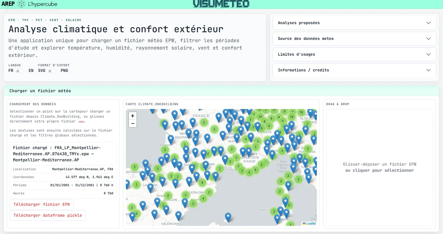
The application allows users to load a local file or select a station from the Climate.OneBuilding index, then apply global month and time-range filters before producing several families of analyses. The outdoor comfort module relies on the calculation of UTCI and PET biometeorological indices, enhanced by a simplified estimate of mean radiant temperature (MRT) and by the inclusion of a dominant surrounding material.

How to use it:

1. Select a weather station.
2. Load the data.
3. Explore the different tabs.
4. Export the charts.

🗂️ Input data and preprocessing

The application handles EPW (EnergyPlus Weather) files representing an hourly meteorological year. In practice, the tool mainly relies on TMYx (Typical Meteorological Year) files provided by Climate.OneBuilding, but it also accepts any EPW file supplied by the user.

The data preparation workflow is as follows:

1. reading the EPW text file;
2. extracting station metadata: name, country, latitude, longitude, time zone;
3. reading the main hourly columns, including: Dry Bulb Temperature, Relative Humidity, Atmospheric Station Pressure, Global Horizontal Radiation, Direct Normal Radiation, Diffuse Horizontal Radiation, Wind Speed, Wind Direction;
4. rebuilding an annual hourly index;
5. adding derived columns useful for the analyses: day of year, hour, date label, day/night, season;
6. optionally applying global filters: month selection and time window, including periods crossing midnight.

An important point is that the year is rebuilt on a single reference year, which makes processing and visual representation easier without introducing ambiguity in the time steps.

📊 Available analyses

The application is not limited to comfort. It brings together four families of analyses sharing the same filtered dataset:

• Temperature / humidity daily averages, monthly averages, typical days by month, annual hourly heatmap.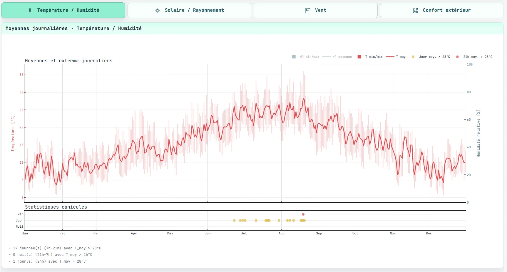

  

• Solar / radiation monthly totals, typical GHI / DHI days, heliodon and annual heatmap of global horizontal radiation.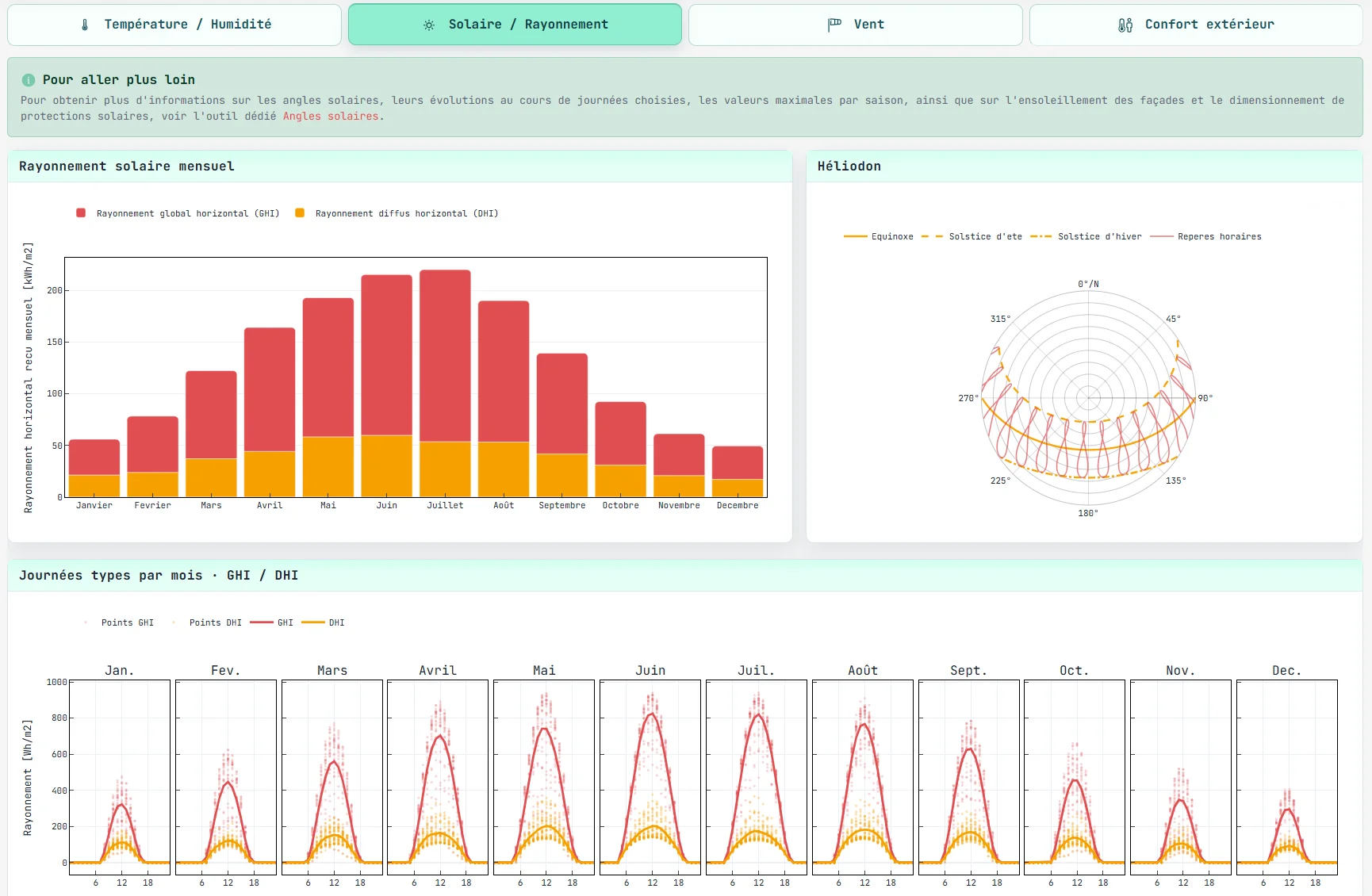

  

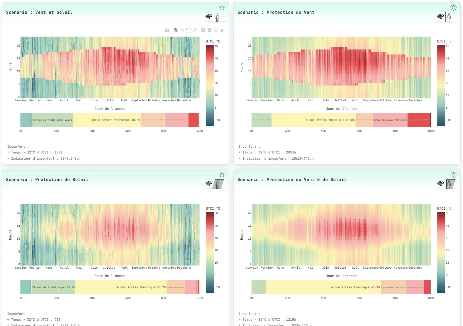
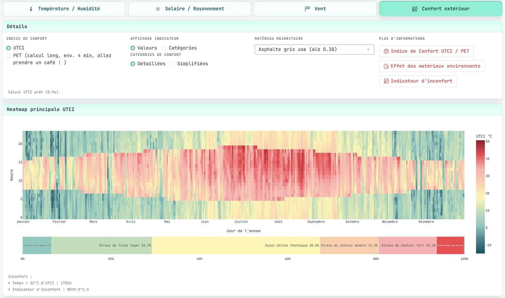
• Wind overall 24h / day / night wind roses and seasonal wind roses.

• Outdoor comfort calculation of UTCI or PET, continuous or categorical display, comparison of four exposure scenarios, discomfort statistics and seasonal comparisons.

This organization keeps weather as the common basis and allows comfort to be read as a combined consequence of air temperature, wind, radiation and a set of surface assumptions.

Visual to insert here: capture of the comfort tab with the four scenarios

☀️ Outdoor comfort calculation logic

The comfort tab computes four typical situations, conceived as project boundary cases:

• WS: wind and sun;
• WNS: wind and shade;
• NWS: sheltered from wind and sun;
• NWNS: sheltered from wind and shade.

The calculation relies on three main ingredients:

• a weather field derived from the EPW file;
• an estimate of MRT depending on solar exposure and dominant material;
• a comfort-index calculation using UTCI or PET.

Computed indices

Two indices are available:

• UTCI (Universal Thermal Climate Index) an outdoor thermal stress index, relatively fast to compute, used by default in the application;
• PET (Physiological Equivalent Temperature) an index expressed in equivalent degrees, numerically more expensive because it is based on a nonlinear physiological resolution.

The computation of both indices is delegated to the pythermalcomfort library, with a few practical assumptions:

• EPW atmospheric pressure is converted from Pa to hPa for the PET calculation,
• pedestrian-level air speed is obtained from weather wind speed through the relation: v_pedestrian = ((1.5 / 10) ^ 0.15) * v_weather;
• a “no-wind” scenario is represented by an imposed speed of 0.15 m/s;
• for the UTCI calculation, speed is bounded to 0.5 m/s to remain compatible with the usual validity range of the model;
• for the PET calculation, the retained minimum speed is 0.1 m/s.

Discomfort indicator

Below the comfort charts, the application displays a discomfort indicator based on:

• the number of hours above a threshold;
• the sum of hourly exceedances in °C.h.

The retained thresholds are:

• UTCI > 32°C;
• PET > 29°C.

This indicator is not a regulatory quantity; it is mainly intended to quickly compare relative situations between scenarios, seasons or materials.

🌡️ Simplified MRT calculation

MRT is treated here as a quantity reconstructed from the weather file, rather than as the result of a detailed geometric simulation. The chosen approach is deliberately lightweight in order to maintain calculation times compatible with an interactive application.

Components taken into account

The calculation distinguishes between:

• direct shortwave radiation;
• diffuse sky radiation;
• radiation reflected by the immediate surroundings;
• a longwave contribution linked to the estimated surface temperature.

Solar position is computed using pvlib, based on the latitude, longitude and time index of the file. From there, the application calculates:

• flux_ortho = DNI / sin(elevation);
• a simplified body projection factor: fproj = 0.233 * cos(elevation) + 0.067;
• the shortwave flux in sun-exposed conditions: SW_sun = flux_ortho * fproj + 0.5 * DHI + 0.5 * albedo * GHI;
• the shortwave flux in shaded conditions: SW_shade = 0.5 * DHI + 0.5 * albedo * GHI.

Direct sun is only taken into account when DNI > 1 W/m² and solar elevation is above 3°. Outside this condition, sun-exposed MRT falls back to air temperature, which avoids introducing a spurious solar effect at dawn, dusk or when no usable direct beam is available.

Retained formulation

MRT is then reconstructed by combining a simplified atmospheric radiative base and additional fluxes:

MRT = ((Ta + 273.15)^4 + (alpha * SW + LW_surface) / (sigma * epsilon_human))^(1/4) - 273.15

with:

• alpha = 0.7: solar absorptivity of the human body;
• epsilon_human = 0.95: radiative emissivity of the human body;
• sigma = 5.67e-8 W/m²/K⁴: Stefan-Boltzmann constant.

This calculation is not intended to reproduce a real urban configuration in detail. It provides a coherent estimate for comparing orders of magnitude and testing the relative effect of shade, wind and materials.

🧱 Materials and the 1R1C model

One specific feature of the tool is the introduction of a dominant surrounding material into the comfort calculation. In the current state of the code, 15 materials are available, covering several families:

• asphalts and bituminous pavements;
• concrete slabs;
• grid pavements;
• sandstones and limestones;
• green or dry grass.

Each material is defined by three parameters:

• an albedo;
• an emissivity;
• a qualitative inertia class.

In the current dataset, albedo values range approximately from 0.05 to 0.68, emissivities from 0.91 to 0.98, and three inertia classes are available:

• low: Ceff = 80 000 J/m²/K
• medium: Ceff = 180 000 J/m²/K
• high: Ceff = 320 000 J/m²/K

Why a 1R1C model?

The retained 1R1C model is a compromise. The objective is not to finely simulate the thermal stratification of a multilayer material, but to represent, at very low computational cost, two effects that matter for outdoor comfort:

• the immediate effect of the material on shortwave exchanges, through albedo;
• the delayed storage and release effect, through a dynamic surface temperature.

In this logic:

• 1R represents a simplified exchange resistance between the surface and the air, mainly through a convective coefficient;
• 1C represents an effective surface heat capacity, that is, the amount of energy that can be stored per unit area and per degree.

Implemented equation

Surface temperature Tsurf is computed hour by hour from air temperature and global horizontal radiation:

Ceff * dTsurf/dt = SW_abs - h_c * (Tsurf - Ta) - LW_net

with:

• SW_abs = (1 - albedo) * GHI
• LW_net = emissivity * sigma * (Tsurf^4 - Ta^4)
• h_c = 8 W/m²/K

The time scheme is explicit:

Tsurf(t+dt) = Tsurf(t) + dt / Ceff * [SW_abs - h_c * (Tsurf - Ta) - LW_net]

and initialization is set to:

Tsurf(t0) = Ta(t0)

A few numerical safeguards are added in the code:

• the time step is inferred from the hourly index, then bounded between 300 s and 7200 s;
• surface temperature is clipped to a band around Ta in order to avoid numerical drift in extreme cases.

Coupling with MRT

Once Tsurf has been estimated, the application computes a net surface longwave flux:

LW_surface = emissivity * sigma * (Tsurf^4 - Ta^4)

This term is then reinjected into the MRT calculation, both in sun and shade. The result is a simple causal chain:

• albedo modifies short-term radiative absorption;
• inertia modulates the heating and phase shift of Tsurf;
• Tsurf in turn modifies the longwave radiative contribution felt by the user.

This architecture makes it possible to reveal comfort differences between materials without resorting to a full ground model.

Visual to insert here: principle diagram of the 1R1C model and its coupling to MRT

⚙️ Assumptions and simplifications to keep in mind

The application relies on several structuring assumptions:

• the weather file is a typical TMYx year, not an exhaustive chronology of extreme conditions or rare occurrences;
• wind is taken from the EPW file and is therefore representative at climatic scale, not necessarily at the local micro-scale;
• shade is modeled by removing direct solar radiation, without explicit masking geometry;
• the “wind shelter” scenario is not simulated through CFD or a local shelter coefficient, but through an imposed residual speed;
• MRT is reconstructed from aggregated fluxes, without a detailed model of views, form factors or urban morphology;
• the surrounding environment is reduced to a single dominant material;
• the 1R1C model represents an equivalent surface rather than a real multilayer assembly.

These simplifications are consistent with the purpose of the tool: compare quickly, test sensitivities and guide design decisions in early project phases.

🧭 Relevant use cases

The application is especially useful for:

• quickly comparing several climates or stations;
• identifying critical periods of heat or discomfort;
• testing the relative effect of shade, wind shelter and ground materials;
• supporting urban or architectural design thinking before a more detailed study.

It is not intended to replace:

• a locally resolved microclimatic study;
• a regulatory energy simulation;
• a fine-scale wind or radiation expertise.

🛠️ Implementation

The application is developed in Python with the Dash framework. The main libraries used are:

• Pandas and NumPy for data processing,
• pvlib for solar position,
• pythermalcomfort for UTCI and PET indices;
• Dash Bootstrap Components for layout and user inputs;
• Dash Leaflet for map display.

The choice of a lightweight architecture keeps response times compatible with exploratory use while still exposing explicit and editable calculation assumptions.