Urban CFD

Turbulence modeling

Comprehensive Approaches

In theory, it is possible to solve any fluid mechanics problem using Navier-Stokes equations . However, this approach (called DNS – Direct Numerical Simulation ), is still far too costly in terms of computing resources and would require extremely fine spatial discretization to be able to capture all the scales of turbulence over the entire zone of interest.

The first way to reduce the necessary computing ressources is to use the method called LES – Large Eddy Simulation . The idea is to simulate (represent) only the largest scales of turbulence (the “largest eddies”), and take into account what happens at the lower scales using models (see figure below). However, many discussions are still ongoing on the optimal type of modelling [Sagaut, 2006]¹.

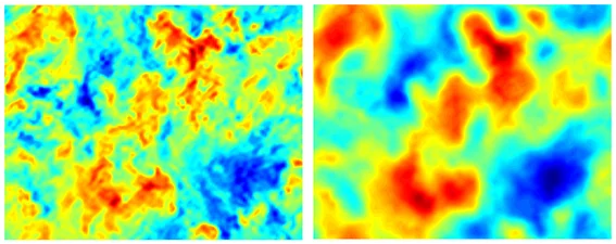
Figure after [Lu, 2008]²

Nowadays, the most widely used method for resolving turbulent flows is the RANS – Reynolds Averaged Navier Stokes [Frank et al., 2004]³. This method time-averages the Navier-Stokes’ equations over all turbulence scales. Similar to the LES methods, it is then necessary to model the effects of turbulence on the mean flow: this is the role of the turbulence models discussed below.

Simulations are performed in Steady State, since the meteorological data is averaged over periods ranging from at least 15 to 30 minutes.

Turbulence Modeling

Within RANS-type approaches, turbulence models aim to define the turbulent variables of the flow as a function of the global variables of the average flow. Two types of approaches exist: one is based on the viscosity of vortices, and derives turbulent stresses from the mean velocity; and the second considers some additional differential equations.

Historically, the most widely used approach remains the linear approach, so-called \(k - \epsilon\):

• \(k\): turbulent kinetic energy,
• \(\epsilon\): rate of dissipation of turbulence energy.

A known problem of this model is the overproduction of turbulent kinetic energy in stagnant areas. Many authors have tried to improve this model, which has generally improved the prediction of pressure coefficients (\(C_{\text{p}}\)), but reduces the quality of velocity predictions, especially behind obstacles.

This model, and the numerous variants that followed can be found below:

• \(k-\epsilon\):
  • Issues with “over production” of kinetic energy in stagnant zones.
• Modified \(k-\epsilon\):
  • Good pressure coefficient assesment near façades, poor velocity prediction downstream of obstacles.
• RNG \(k-\epsilon\) (ReNormalization Group) or Realizable \(k - \epsilon\):
  • Mitigation of stagnation problems
  • Better results downstream of obstacles,
  • Seems to work best for simulating complex environments (many buildings).
• SST \(k-\omega\) (Shear Stress Transport):
  • A priori, the best variant of the \(k-\epsilon\).

Overall, all linear models suffer from the isotropy hypothesis of Reynolds normal stresses. Non-linear models should be used in theory, but still too few applications exist to date.

In summary, it is better to avoid the \(k-\epsilon\) model as is,and use at least the Realizable \(k-\epsilon\), or even better the SST \(k-\omega\). In the case of several building modeling, the RNG \(k-\epsilon\) model seems to yield correct results.

Atmospheric Boundary Layer

Origins

When a fluid flows along a stationary wall, the velocity on the wall is zero, while far from the wall they are equal to the velocity of the undisturbed flow, as shown in Figure 2. This velocity gradient zone is called Boundary Layer.

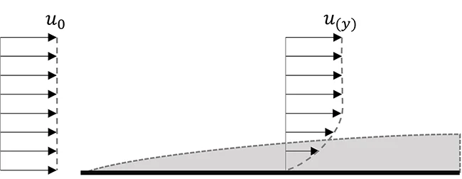
According to a surface normal, the speed will therefore vary between 0 [m.s^-1] and a given maximum. The velocity variation depends on the viscosity of the fluid that induces friction between adjacent layers.

The boundary layer is defined as the region of the flow where viscous effects are at least as important as inertial effects. In general terms, we define \(\Delta (x)\) as the thickness of the boundary layer, such that:

$$ u\left( \Delta (x) \right) = 0.99 \times u_{\text{inf}} $$

where \(u_{\text{inf}}\) is the maximum velocity (in the undisturbed flow), as shown in Fig. 3.

Definitions

The Atmospheric Boudary Layer (ABL) represents the part of the atmosphere directly influenced by the effects of the Earth’s surface (continental or oceanic). Beyond this area, the influence of the ground is considered negligible. This layer can be roughly divided into 3 layers, as shown in Fig. 3 (modified after [Grazzini, 1999]⁴).

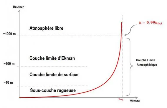
The first rough sublayer in the immediate vicinity of the ground is a zone where the wakes of obstacles encountered by the wind are mixed. The velocity fields are very disturbed, and friction forces are predominant. Its thickness can vary from a few millimetres (sea surface) to about ten metres (urban areas).

Immediately above it is the Surface Boundary Layer (SBL), also known as the mixing layer or Prandtl layer. It is defined as the region where the temperature decreases rapidly during the day with altitude, and more generally as the region where the fluxes of momentum and heat (sensitive and latent) are conservative and equal to those of the ground. Within this area, turbulence is homogeneous, and the wind direction does not vary (or only slightly) with altitude. Velocity, on the other hand, varies in proportion to the logarithm of altitude. It represents about 10% of the ABL, and extends over heights ranging from ten to a hundred meters.

Finally, there is the Ekman layer (also called the dynamic boundary layer), where the Coriolis force (induced by the rotation of the earth) becomes comparable to the friction forces on the ground. This leads to deviations in wind direction with altitude, which can reach 30 to 40° in the anticyclonic direction (to the right in the northern hemisphere, and to the left in the southern hemisphere).

Characterization

The representation of the average wind profile is based on results from fluid mechanics. In practice, two types of profiles are used, one follows a logarithmic and the other a power law, depending on the altitude \(z\).

Logarithmic profile

Although there is no exact description of this ABL to date, many approximations exist. The most common, recommended by different authors (e.g. [Frank et al, 2004]³ or [Blocken et al., 2012]⁵) is the description proposed by [Richards et al., 1993]⁶. This assumes zero vertical velocity, constant pressure in the vertical direction and flow direction, and constant shear stresses in the ABL. Thus the vertical velocity profile can be obtained by the following logarithmic law:

$$ U(z)=\frac{u_*}{K} \ln \left( \frac{z+z_0}{z_0}\right) $$

where \(U(z)\) is the speed at an altitude \(z\), \(z_0\) is the surface roughness, \(K\) the von Karman constant (usually the value is around 0.4), and finally \(u_*\) the speed of friction. The latter is obtained by the relationship:

$$ u_* = \frac{KU_h}{\ln \left( \frac{h+z_0}{z_0} \right)} $$

It is calculated from the reference speed \(U_h\) measured at an altitude \(h\). This is typically the value measured in weather stations at a height of 10 m.

Power law profile

In some cases, for simplicity’s sake, a simpler approximation can be used and allows a faster evaluation of flow rates as a function of height. This is the “power law”, which is expressed as follows:

$$ \frac{u(z)}{u_0} = \left( \frac{z}{H_0} \right)^m $$

Where \(u_0\) is the air flow velocity measured at a height \(H_0\), \(z\) is the altitude and finally a parameter that characterizes the profile distortion. Its value is usually between 0.1 and 0.2.

Note : There is no mathematical justification for the validity of this law, however it seems to be in adequacy with the measured experimental profiles, especially after adjusting the parameter \(m\).

Turbulence of the ABL

When using 2-equations turbulence models (the most commonly used), the values and \(k\) and \(\epsilon\) are also obtained with the ABL hypothesis. The formulas for determining them can be found in [Ricahards et al., 1993]⁶ and are the result of conservation equations.

Law of the wall

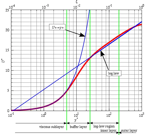
Figure source: Law of The Wall

The boundary layer close to the walls is divided into three zones characterized by the dimensionless distance to the wall \(y^+\) defined such follow: \(y^+=\frac{U^+ y}{\nu}\) where \(U^+\) is the shear velocity \(\nu\), the kinematic viscosity and \(y\) the wall distance. These three zones, illustrated on Fig. 5, are:

• the viscous sub-layer: in a zone where \(0\le y^+<5\) the viscous effect are predominant,
• the buffer zone where \(y^+\) is as follow \(5<y^+<30\),
• Finaly, the logaritmic layer with \(y^+\) ranging from 30 to 300. In this area, turbulent effects are predominant and the velocity follows a logarithmic law defined by:

$$ U^+=\frac{1}{\kappa}\log y^+ + C $$

There are two approaches commonly used in CFD to model turbulence i near wall areas. On the one hand, there are “low Reynolds number” turbulence models that calculate the flow variables throughout the boundary layer. The disadvantage of this method is that it requires a very fine mesh size with first mesh cells located in the viscous sublayer On the other hand, there are so-called “high Reynolds number” turbulence models that model the flow in the boundary layer via the logarithmic law. The result’s accuracy near the wall is then reduced, but these methods are reduce considerably the calculation times.

Urban CFD recommandation

Modeling area

If we are interested in a building with a height of \(H\), it is advised to model the lateral faces and the upper face at a minimum distance of \(5H\). Ideally on the downstream side, it is advisable to model a distance of \(15H\) [Frank et al., 2004]³, [Tominaga et al., 2008]⁷. The purpose of the increased distance downstream of the object of study is to have “enough” space to obtain a stable flow.

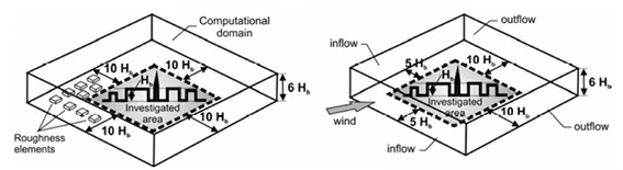
Figure after [Frank, 2007]⁸

In general, the “blockage ratio” (ratio of surfaces between the projection of the object of study and the upstream side) must be less than 10%, and ideally around 3 to 5%.

Discretization

Global recommendation

• In general, it is preferable to use prismatic (rather than tetrahedral) elements.
• Except in special cases, in order to limit numerical diffusion problems, the mesh should be built in the wind axis.
• For all modelled buildings, it is necessary to have at least 10 mesh cells per dimension.
• For “streets” (space between 2 neighbouring buildings), it is necessary to have a minimum of 6 to 8 mesh cells ( < 2m) in order to be able to represent the air jets, as well as possible wall detachments.
• In the case where the urban environment is also modelled, the “other” buildings must have at least 3 meshes cells in all directions
• The vertical resolution must be fine (\(\delta \lt 10\) m) up to a height of \(3H\).
• The vertical resolution must be fine near the ground, especially if we are interested in pedestrian comfort (2m).

Specific recommendations for the buildings of interest

• On the roof, and near the edges (corners) of the building, the mesh size must be “thin enough” to be able to represent wall indentations and recirculation areas. (\(\delta < \frac{L_{\text{max}}}{10}\)) .
• Overall, we want increasingly fine mesh sizes as the building approaches, however the expansion factor must remain below 1.2 - 1.3 near the surfaces (ratio between the sizes of 2 adjacent cells).