Piston effect in underground networks

The symbols used hereafter are explained in the nomenclature located at the end of this page.

Understanding air flows and overpressure in underground stations is necessary to be able to assess reliably the user comfort. As part of the work carried out on air quality in underground stations , the objective is to estimate the order of magnitude of the quantity of air which is displaced with a given train station following the arrival and departure of a train.

Concept of pressure losses

When a fluid is moving in a duct, part of its energy is dissipated by friction leading to a pressure drop. Two types of pressure drops exist:

The pressure loss due to friction in a straight pipe of the same length. This can be modelled with Darcy’s law as follows:

$$ \Delta P =\frac{\rho\lambda Lv^2}{2D_{\text{h}}} $$

Where $P$ is the pressure, $v$ the fluid velocity, $L$ is the duct length, $D_{\text{h}}$ is the hydraulic diameter and $\lambda$ the pressure drop coefficient.

The pressure loss due to any change in the pipe geometry (section area, bended pipe, T-junction, …). This can be modelled via a coefficient $\xi$ that can be estimated, for example, using Idelchik tables ¹.

The total pressure loss in a pipe with a change in geometry can then be written as the sum of the two types of pressure losses aformentioned as follows:

$$ \Delta P_\text{tot} =\frac{\rho v^2}{2 }\left(\frac{ \lambda L }{D_{\text{h}}}+\xi\right) $$

Equation governing the phenomenon

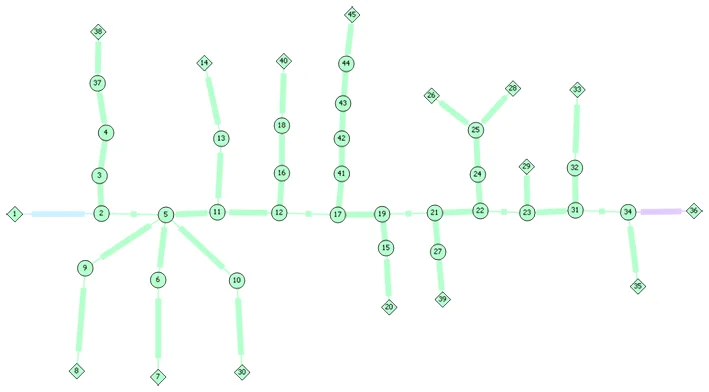
The calculation of the piston effect in an underground station requires modelling a network of tunnels in which a train will move along a linear path and mark a certain number of stops. It is therefore a question of modelling transient 1D flows, driven by the pressure drop induced by the train motion.

réseau aeraulique souterrin — *Example of an underground network (SPES1D-AREP software)*

The equations used to establish this simplified model are based on the principles of conservation of mass and quantity of motion (recalled here ). By solving these equations, it is possible to calculate the velocity of the air put into motion by the train.

For this purpose, the generalized Bernouilli theorem is applied to a fluid control volume surrounding the train.

effet piston souterrain — *Illustration of the piston effect*

This yields to the following equation for the air flow in the tunnel:

$$ \rho C \frac{\mathrm{d}Q_{\text{s}}}{\mathrm{d}t} = \underbrace{\Delta P_{\text{sing}} + \Delta P_{\text{lin}} + \Delta P_{\text{fan}} + \Delta P_{\text{piston}} }_{w(Q_{\text{s}})}+\Delta P_{\text{ext}} $$

Where $\Delta P_\text{sing}$ corresponds to the pressure difference generated at any change in section (especially at the front and rear of the train), $\Delta P_\text{lin}$ corresponds to the pressure difference induced by friction in a constant cross-section duct, $\Delta P_\text{fan}$ corresponds to the pressure difference due to mechanical ventilation, $\Delta P_\text{piston}$ corresponds to the pressure difference caused by the piston effect caused by the train motion and $\Delta P_\text{ext}$ is the pressure difference between the two ends of the tunnel of interest.

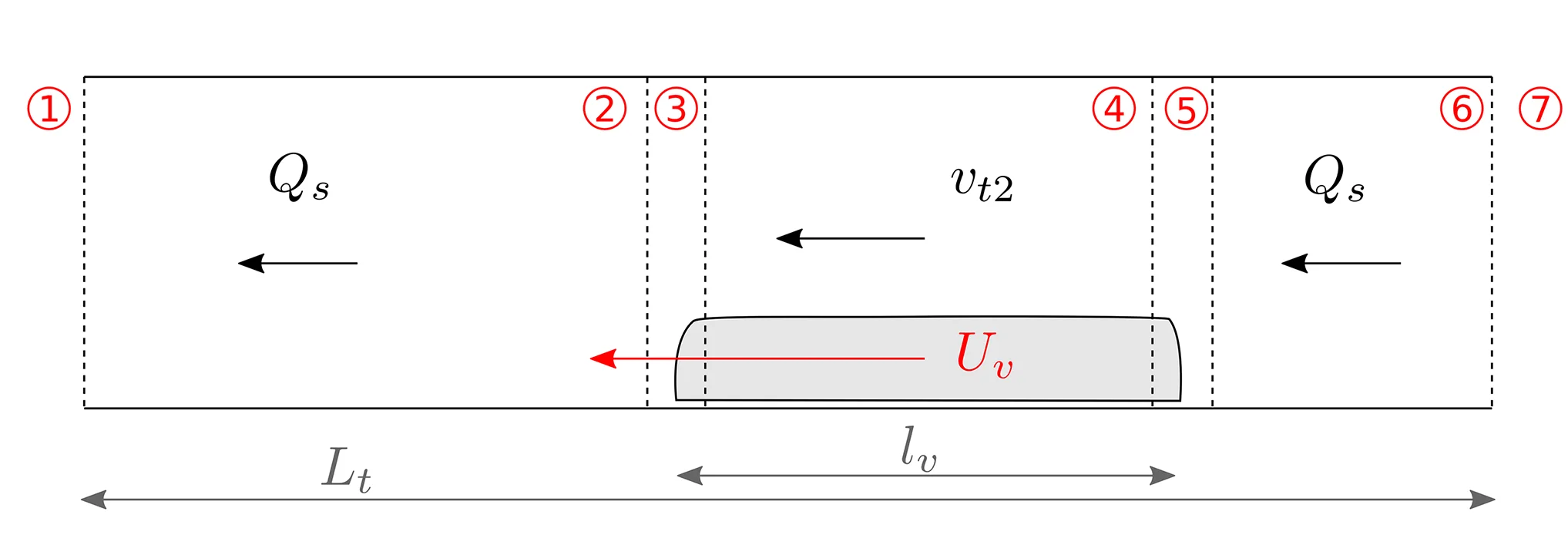
$C$ is the term corresponding to the inertia of the air column::

With a train: $C=\frac{L_{\text{t}}}{A_{\text{t}}}$
Without a train: $C=\frac{L_{\text{t}}-l_{\text{v}}}{A_{\text{t}}}+\frac{l_{\text{v}}}{A_{\text{t}}-a_{\text{v}}}$

Let $L_{\text{t}}$ be the length of the tunnel segment, $l_{\text{v}}$ the length of the vehicle located in the tunnel, $A_{\text{t}}$ the section of the tunnel segment and $a_{\text{v}}$ the section of the vehicle in the segment.

The state-of-the-art provides the following expressions for the different pressure losses $\Delta P$ as shown in the following table:

	Without train	With Train
$\Delta P_\text{lin}$	$-\frac{\rho f_{\text{t}} L_{\text{t}} P_{\text{t}} \mid Q_{\text{S}} \mid Q_{\text{S}}}{8 A_{\text{t}}^3}$	$ -\frac{\rho f_{\text{t}} L_{\text{t}} P_{\text{t}} \mid Q_{\text{S}} \mid Q_{\text{S}}}{8 A_{\text{t}}^3} $
$\Delta P_\text{sing}$	$-k\rho\frac{\mid Q_{\text{S}} \mid Q_{\text{S}}}{2 A_{\text{t}}^2}$	$-k\rho\frac{\mid Q_{\text{S}} \mid Q_{\text{S}}}{2 A_{\text{t}}^2}$
$\Delta P_\text{fan}$	$\rho\frac{ \mid Q_\text{fan}\mid \left(v_\text{fan}-\frac{Q_{\text{S}}}{A_{\text{t}}}\right)}{A_{\text{t}}}$	$\rho\frac{ \mid Q_\text{fan} \mid \left(v_\text{fan}-\frac{Q_{\text{S}}}{A_{\text{t}}}\right)}{A_{\text{t}}}$
$\Delta P_\text{piston}$	$0$	$\frac{\rho (\textcolor{limegreen}{K_{\text{vB}}}+\textcolor{red}{K_{\text{vF}}})(A_{\text{t}} U_{\text{v}}-Q_{\text{S}})^2}{2 A_{\text{t}}^2} + \frac{\rho f_{\text{t}} l_{\text{v}} P_{\text{t}} \mid (a_{\text{v}} U_{\text{v}}-Q_{\text{S}})\mid (a_{\text{v}} U_{\text{v}}-Q_{\text{S}})}{8 (A_{\text{t}}-a_{\text{v}})^3}+\frac{\rho \lambda_{\text{v}} l_{\text{v}} P_{\text{v}} \mid (a_{\text{t}} U_{\text{v}}-Q_{\text{S}})\mid (a_{\text{t}} U_{\text{v}}-Q_{\text{S}}) }{8 (A_{\text{t}}-a_{\text{v}})^3}+\frac{\rho a_{\text{v}} l_{\text{v}}}{A_{\text{t}}-a_{\text{v}}}\frac{dU_{\text{v}}}{dt} \textcolor{limegreen}{+\rho \frac{Q_{\text{S}}^2}{2 A_{\text{t}}^2}-\rho\frac{(a_{\text{v}} U_{\text{v}}-Q_{\text{S}})^2}{2 (A_{\text{t}}-a_{\text{v}})^2}}\textcolor{red}{-\rho\frac{Q_{\text{S}}^2}{2 A_{\text{t}}^2}+\rho\frac{(a_{\text{v}} U_{\text{v}}-Q_{\text{S}})^2}{2 (A_{\text{t}}-a_{\text{v}})^2}}+\frac{\rho f_{\text{t}} l_{\text{v}} P_{\text{t}} \mid Q_{\text{S}}\mid Q_{\text{S}}}{8 A_{\text{t}}^3}$

Red terms must be taken into account when the front of the train is located in the tunnel of interest. The blue terms must be introduced when the rear of the train located in the tunnel of interest.

Note :
In steady-state and in the absence of a train, the equation governing the air flow can be written as:
$$ \Delta P = Z Q_{\text{s}}^2 $$

This equation is commonly used for the study of hydraulic networks using the “Z method” but given the importance of the transient effects produced by the passage of the train, this method is not applicable in this context.

Network resolution

Considering that the equations governing the air flow are now established for all the tunnels of the network, they are reorganised to form the following system of equations:

$$ \rho\left[\underline{\underline{C}}\right]\cdot\left[\underline{\dot{Q_{\text{s}}}}\right]=\left[\underline{\omega}(Q_{\text{s}})\right] $$

To do this, we use the node and mesh methods (similar to those used in electrical engineering) illustrated below:

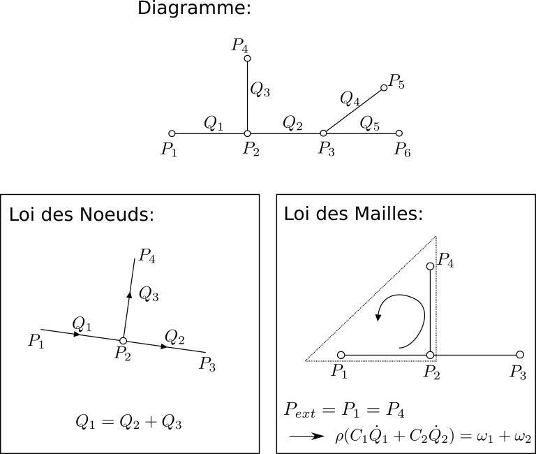
diagramme maille noeud resolution — *Diagram of nodes and links*

The transient system can then be solved by using a explicit resolution scheme .

Presentation of SPES1D

A software named SPES1D (for Subway Piston Effect Simulation in 1D) was developed by our experts to solve the transient air flow caused by trains operating in tunnels and underground stations.

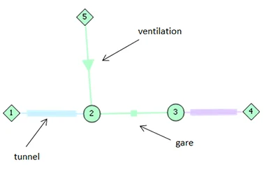
This software introduces three categories of segments to cover a wide range of cases:

the duct-type element. This is the most basic element. It can be used both for tunnels, stations (if the train does not stop) and various ducts (junctions between two passenger buildings, underground passages,…),
the station-type element. This element is used for stations where the train stops. For this element, when the train is stopped, the centre of the station coincides with the centre of the train,
the fan-type element with ventilation. This element accounts for the effects of mechanical ventilation.

SPES elements — *Various 'blocks' available in SPES1D*

It is then possible to determine, during the train motion, the change in velocity and pressure in each element constituting the network.

debit aeraulique train entree gare — *Calculated flow rate while the train passes at the station entrance*

debit aeraulique train sortie gare — *Calculated flow rate at the train station exit while the train passes*

Validation

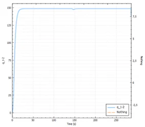
The software developed, SPES1D, was validated after comparison with [Sajben, 1971]² study. In his article, Sajben studied the piston effect of a train with a constant propulsive power. Among others, e observed a given set-up that when the train reaches 21 m/s, the air in the tunnel is moved at 8.2 m/s. The same set-up was modelled and simulated with our in-house software SPES1D. Under the same operating conditions and for a train also moving at 21 m/s, the speed of the displaced air also reached 8.2 m/s.

Nomenclature

Symbole	Signification
$A$	Section [m²]
$A_{\text{t}}$	Tunnel section [m²]
$a_{\text{v}}$	Train section [m²]
$C$	Inertial term of the air column
$D_H$	Hydraulic diameter [m]
$K_{\text{vB}}$	Coefficient of sudden pressure drop due to air expansion following the passage of the train
$K_{\text{vF}}$	Coefficient of sudden pressure drop due to air contraction as the train passes through
$P$	Pressure [Pa]
$\Delta P_{\text{ext}}$	Pressure difference between the ends of the segment [Pa]
$\Delta P_{\text{sing}}$	Pressure variation within a change in geometry [Pa]
$\Delta P_{\text{lin}}$	Pressure difference due to friction [Pa]
$\Delta P_{\text{fan}}$	Pressure difference induced by mechanical ventilation [Pa]
$\Delta P_{\text{piston}}$	Pressure difference induced by piston effect [Pa]
$f_{\text{t}}$	Pressure drop coefficient for the tunnel [Pa]
$L$	Length [m]
$L_{\text{t}}$	Tunnel length [m]
$l_{\text{v}}$	Train length [m]
$\lambda$	Regular pressure drop coefficient
$\lambda_{\text{v}}$	Pressure drop coefficient at the train level
$Q$	Flow rate [kg/m³]
$Q_{\text{s}}$	Air flow rate due to the piston effect [kg/m³]
$U_{\text{v}}$	Train speed [m/s]
$v$	Air velocity [m/s]
$\rho$	Air density [kg/m³]
$Z$	Hydraulic resistance
$\xi$	Singular pressure drop coefficients

Idelchik, I. E., 1986, Handbook of hydraulic resistance. Washington. PDF link ↩︎
Sajben, M. (1971). Fluid Mechanics of Train-Tunnel Svstems in Unsteady Motion. AIAA Journal, 9(8), 1538-1545. DOI ↩︎

	Without train	With Train
\(\Delta P_\text{lin}\)	\(-\frac{\rho f_{\text{t}} L_{\text{t}} P_{\text{t}} \mid Q_{\text{S}} \mid Q_{\text{S}}}{8 A_{\text{t}}^3}\)	\( -\frac{\rho f_{\text{t}} L_{\text{t}} P_{\text{t}} \mid Q_{\text{S}} \mid Q_{\text{S}}}{8 A_{\text{t}}^3} \)
\(\Delta P_\text{sing}\)	\(-k\rho\frac{\mid Q_{\text{S}} \mid Q_{\text{S}}}{2 A_{\text{t}}^2}\)	\(-k\rho\frac{\mid Q_{\text{S}} \mid Q_{\text{S}}}{2 A_{\text{t}}^2}\)
\(\Delta P_\text{fan}\)	\(\rho\frac{ \mid Q_\text{fan}\mid \left(v_\text{fan}-\frac{Q_{\text{S}}}{A_{\text{t}}}\right)}{A_{\text{t}}}\)	\(\rho\frac{ \mid Q_\text{fan} \mid \left(v_\text{fan}-\frac{Q_{\text{S}}}{A_{\text{t}}}\right)}{A_{\text{t}}}\)
\(\Delta P_\text{piston}\)	\(0\)	\(\frac{\rho (\textcolor{limegreen}{K_{\text{vB}}}+\textcolor{red}{K_{\text{vF}}})(A_{\text{t}} U_{\text{v}}-Q_{\text{S}})^2}{2 A_{\text{t}}^2} + \frac{\rho f_{\text{t}} l_{\text{v}} P_{\text{t}} \mid (a_{\text{v}} U_{\text{v}}-Q_{\text{S}})\mid (a_{\text{v}} U_{\text{v}}-Q_{\text{S}})}{8 (A_{\text{t}}-a_{\text{v}})^3}+\frac{\rho \lambda_{\text{v}} l_{\text{v}} P_{\text{v}} \mid (a_{\text{t}} U_{\text{v}}-Q_{\text{S}})\mid (a_{\text{t}} U_{\text{v}}-Q_{\text{S}}) }{8 (A_{\text{t}}-a_{\text{v}})^3}+\frac{\rho a_{\text{v}} l_{\text{v}}}{A_{\text{t}}-a_{\text{v}}}\frac{dU_{\text{v}}}{dt} \textcolor{limegreen}{+\rho \frac{Q_{\text{S}}^2}{2 A_{\text{t}}^2}-\rho\frac{(a_{\text{v}} U_{\text{v}}-Q_{\text{S}})^2}{2 (A_{\text{t}}-a_{\text{v}})^2}}\textcolor{red}{-\rho\frac{Q_{\text{S}}^2}{2 A_{\text{t}}^2}+\rho\frac{(a_{\text{v}} U_{\text{v}}-Q_{\text{S}})^2}{2 (A_{\text{t}}-a_{\text{v}})^2}}+\frac{\rho f_{\text{t}} l_{\text{v}} P_{\text{t}} \mid Q_{\text{S}}\mid Q_{\text{S}}}{8 A_{\text{t}}^3}\)

Symbole	Signification
\(A\)	Section [m²]
\(A_{\text{t}}\)	Tunnel section [m²]
\(a_{\text{v}}\)	Train section [m²]
\(C\)	Inertial term of the air column
\(D_H\)	Hydraulic diameter [m]
\(K_{\text{vB}}\)	Coefficient of sudden pressure drop due to air expansion following the passage of the train
\(K_{\text{vF}}\)	Coefficient of sudden pressure drop due to air contraction as the train passes through
\(P\)	Pressure [Pa]
\(\Delta P_{\text{ext}}\)	Pressure difference between the ends of the segment [Pa]
\(\Delta P_{\text{sing}}\)	Pressure variation within a change in geometry [Pa]
\(\Delta P_{\text{lin}}\)	Pressure difference due to friction [Pa]
\(\Delta P_{\text{fan}}\)	Pressure difference induced by mechanical ventilation [Pa]
\(\Delta P_{\text{piston}}\)	Pressure difference induced by piston effect [Pa]
\(f_{\text{t}}\)	Pressure drop coefficient for the tunnel [Pa]
\(L\)	Length [m]
\(L_{\text{t}}\)	Tunnel length [m]
\(l_{\text{v}}\)	Train length [m]
\(\lambda\)	Regular pressure drop coefficient
\(\lambda_{\text{v}}\)	Pressure drop coefficient at the train level
\(Q\)	Flow rate [kg/m³]
\(Q_{\text{s}}\)	Air flow rate due to the piston effect [kg/m³]
\(U_{\text{v}}\)	Train speed [m/s]
\(v\)	Air velocity [m/s]
\(\rho\)	Air density [kg/m³]
\(Z\)	Hydraulic resistance
\(\xi\)	Singular pressure drop coefficients