The \(Z\) method

It is often useful to use simplified approaches to calculate flows and pressures in a network rather than implementing a heavy, complex and expensive fluid mechanics calculation. The so-called \(Z\) method, or hydraulic impedance method (by electrical analogy) for calculating fluid flows in a system of nodes and branches, is presented here. Pressures play the role of potential while flows represent intensity.

Governing equation

Between two points of a flow, the Bernoulli equation governing the linear pressure drop, related to the linear friction coefficient \(\lambda\) as well as singularties (\(\xi\) factor) is the following:

$$ \Delta p = \frac{\rho v^2}{2} \times \Big (\frac{\lambda L}{D_{\text{h}}} + \xi \Big ) \text{ [Pa]} $$

If we express it as a function of flowrate \(Q_{\text{v}}\) in a pipe of sectional area \(S\) we obtain:

$$ v^2 = \frac{2}{\rho} \Delta p \times \Big (\frac{\lambda L}{D_{\text{h}}} + \xi \Big )^{-1} \text{ [m²/s²]} $$

$$ Q_{\text{v}}^2 = \frac{2 S^2}{\rho (\frac{\lambda L}{D_{\text{h}}} + \xi)} \Delta p $$

the following expression then appears for the flow rate:

$$ Q_{\text{v}} = S\sqrt{\frac{2}{\rho(\frac{\lambda L}{D_{\text{h}}} + \xi)} } \sqrt{\Delta p} \text{ [m3/s]} $$

The so-called “Z” method consists in expressing the pressure drop in the form of \(\Delta p = Z \times Q_{\text{v}}^2\), which resembles Ohm’s law ). In this case it is equivalent to:

$$ \Delta p = \frac{\rho(\frac{\lambda L}{D_{\text{h}}} + \xi)}{2S^2} \times Q_{\text{v}}^2 \text{ [Pa]} $$

Then the “hydraulic resistance” (or aeraulic) is defined as \(Z\):

$$ Z = \frac{\rho}{2S^2} \Big (\frac{\lambda L}{D_{\text{h}}} + \xi \Big ) \text{ [Pa.s²/m}^6\text{]} $$

Integration of the discharge coefficient \(C_{\text{d}}\)

A frequently used quantity in aeraulics is the discharge coefficient \(C_{\text{d}}\) which gives the reduction in flow caused by the passage of an orifice due to the constriction of the jet, in particular by inertial effects, and viscous friction. It should be noted that the value of this coefficient is questionable - see section 2 of this page .

If we want to convert the discharge coefficient of an opening into a pressure drop, we must go back to the definition of the problem and calculate the equivalent aeraulic resistance \(Z\) from the equation between \(Q_{\text{v}}\) and \(C_{\text{d}}\) :

$$ Q_{\text{v}} = C_{\text{d}} S \sqrt{ \frac{2 \Delta p}{\rho}} $$

In order to be able to write “fluxes equality” in a form allowing the calculation of the equivalent air resistance, the previous equation is transformed into:

$$ Q_{\text{v}}^2 = \frac{2 (C_{\text{d}} S)^2 }{\rho}\Delta p $$

Yielding an equivalent \(Z\) such that:

$$ Z = \frac{\rho}{2 (C_{\text{d}} S)^2 } $$

For serial air resistance it will be sufficient to add the \(Z\) of each element. For example, the equivalent \(Z\) combining linear and singular pressure losses \( (\lambda, \xi)\) as well as the flow reduction related to a discharge coefficient \(C_{\text{d}}\) of an opening is:

$$ Z_\text{eq} = \frac{\rho}{2S^2} \Big (\frac{\lambda L}{D_{\text{h}}} + \xi + \frac{1}{C_{\text{d}}^2} \Big ) $$

We are therefore able to equate a system governing the balance of pressures and flows: it is now a question of writing it down and solving it!

Non-linear system of equations

When several nodes are at different pressures \(p_i\) and we want to know the pressure \(p\) in the middle point as well as the flow rates \(Q_{\text{v}i}\) between nodes as presented on following figure.

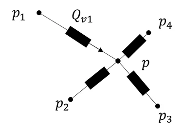
We must therefore resolve the balances of pressures and flows as well as the conservation of mass (the algebraic sum of flows is zero). This gives us the following non-linear system where \(p\) and the \(Q_{\text{v}i}\) are the unknowns:

$$ (p_1 - p) = Z_1 Q_{\text{v}1}^2 $$

$$ (p_2 - p) = Z_2 Q_{\text{v}2}^2 $$

$$ (p_n - p) = Z_n Q_{\text{v}n}^2 $$

$$ Q_{\text{v}1} + … +Q_{\text{v}n} = 0 $$

This raw resolution does not always converge because in some cases there is no solution such that the central pressure is between the bounds of the external pressures. This is due to the fact that the squared flow formulation reduces the space of solutions to those that are positive. However, the problem could be overcome by keeping the same system, provided that \(Z_i\) takes the sign of \(Q_{\text{v}i}\).

Following system, where the flow rates \(Q_{\text{v}i}\) are not risen to the power of two, is a simple way to leave the sign of solutions free (note the trick of the absolute value of the root):

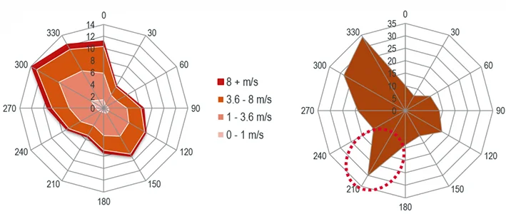
$$ \frac{p_1-p}{\sqrt{|p_1 - p|}} = \sqrt{Z_1} Q_{\text{v}1} $$

$$ \frac{p_2-p}{ \sqrt{|p_2 - p|}} = \sqrt{Z_2} Q_{\text{v}2} $$

$$ \frac{p_n-p}{ \sqrt{|p_n - p|}} = \sqrt{Z_n} Q_{\text{v}n} $$

$$ Q_{\text{v}1} + … +Q_{\text{v}n} = 0 $$

An example of an application is given in the figure below: from the wind rose (left), the pressures on the facade of a building are calculated and then the resulting flow rose (right), using the method described in this article.