Wind Driven Rain
Introduction
The phenomenon of pouring rain corresponds to the combination of the effects of rain with those of the wind. This phenomenon can be the cause of various issues such as:
- Rain penetration [Peerez-Bella et al. 2013]1,
- Damage caused by freezing [Frank et al. 1995]2 [Zhou et al. 2020]3,
- Salt efflorescence-induced discoloration [Granneman et al. 2019]4,
- Structural cracking due to thermal and humidity gradients [Annila et al, 2017]5[Slusarek, 2020]6,
- and the soiling of facades through material leaching [Blocken et al., 2013]7.
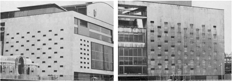
Figure after [White, 1967]8
In this article, we present a method for evaluating a building’s exposure to rain in its urban environment using Computational Fluid Dynamics (CFD). This will make it possible to determine the risks to which facades are exposed and to implement preventive solutions or assess their effectiveness.
We will not delve into the physics of clouds and raindrops, surface phenomena such as splashing, runoff, evaporation, and absorption, the mechanisms of rain penetration into buildings, or the development and execution of waterproofing tests.
First, we will revisit the meteorological phenomenon of rain. Then, we will explore how the combination of “rain + wind” is modeled. We will subsequently present a case study on which we will conduct a sensitivity analysis.
The meteorological phenomenon of rain
Definitions
Rain is the phenomenon by which liquid water droplets fall from clouds to the ground. It is the most common form of precipitation on Earth. When the diameter of the droplets is less than \(\phi\) = 0.5 mm, the precipitation is called drizzle.
The volume of precipitation that reaches a specific area over a certain period of time is characterized by its intensity. Therefore, the intensity of rain is expressed in millimeters per hour [mm/h] or liters per square meter per hour [l/m²/h].
Rain drops size and shape distribution
The water droplets that make up rain can vary in shape and size during a rain episode.
Shape
The droplets tend to be more spherical for small diameters. In contrast, larger droplets appear more like oblate spheroids.

Figure after [Beard et al., 2010]9
This variation in shape has significant consequences for the terminal falling velocity of water droplets.
So, in the absence of wind, a water droplet will only be subjected to the drag force \(\bar{f}_{\text{D}}\) and the gravitational force \(\bar{f}_{\text{G}}\) given by:
$$ \left|\left|\bar{f}\_{\text{G}}\right|\right| = \rho g \pi \frac{\phi^3}{6} \text{~~~~~(1)} $$$$ \left|\left|\bar{f}\_{\text{D}}\right|\right| = \frac{1}{2} \rho A C_{\text{d}} \ V^2 $$Where \(\rho\) is the density of water, \(g\) is the acceleration due to gravity, \(\phi\) is the diameter of the droplet, \(A\) is the cross-sectional area presented by the droplet to the flow, \(C_{\text{d}}\) is the drag coefficient, and \(V\) is the falling velocity.
When \(\left|\left|\bar{f}_{\text{G}}\right|\right| \ll \left|\left|\bar{f}_{\text{D}}\right|\right|\), the droplet accelerates, and the falling velocity increases until it reaches a terminal velocity, $V\_{\text{t}}=\sqrt{\frac{2 \left|\left|\bar{f}\_{\text{G}}\right|\right|}{\rho A C_{\text{d}}}}$ when $\left|\left|\bar{f}\_{\text{G}}\right|\right| = \left|\left|\bar{f}\_{\text{D}}\right|\right|$.
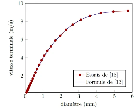
The authors of [Gunn et al. 1949]10 conducted experiments that allowed them to plot the red curve in the previous figure. It can be observed that for droplets with a diameter exceeding 4mm, the terminal velocity does not increase significantly with an increase in volume. This trend can be explained by the change in the droplet’s shape. In fact, an oblate spheroid increases the drag force, which then increases faster than the effects of gravity as the diameter increases. Thus, four-millimeter and six-millimeter droplets exhibit similar terminal velocities.
The authors of [Dingle et al., 1972]11 provide an analytical expression that allows for the straightforward calculation of the terminal velocity of water droplets as a function of their diameter \(\phi\):
$$ V_{\text{t}}(\phi) = -0.166033+4.91844 \phi -0.888016 \phi^2 +0.054888 \phi^3 \text{~~~~~(2)} $$This equation, accurate to within \(\pm\)2%, is valid for diameters in the range of \(\phi \le\) 5.8 mm (blue curve, figure 3).
Size
Raindrops not only exhibit a wide variety of shapes but also a broad range of sizes.
It is commonly accepted in the scientific community that the distribution of droplet sizes can be approximated by a function of rain intensity.
Numerous researchers, such as [Laws et al., 1943]12 [Marshall et al. 1948]13 [Best, 1950]14 [Fujiwara, 1961]15 have conducted measurements and developed their own models. They demonstrated that the sought-after distribution also varies depending on the type of storm and cloud height. However, we can rely on the work of [Best, 1950]14, who proposed an expression for the cumulative probability distribution of droplet sizes as a function of rain intensity.
$$ \left(\theta\right) = 1-\exp\left[-\left(\frac{\phi}{A r_{\text{h}}^p}\right)^n\right] \text{~~~~~(3)} $$Where $r_{\text{h}}$ is the rain intensity, $A$ , $p$ and \(n\) are constants that can be taken equals to average valuess $A$=1.30, $p$=0.232 and $n$=2.25 as computed by [Best, 1950]14.
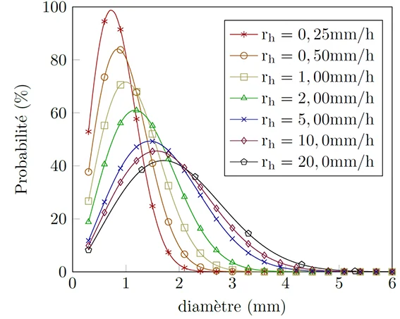
Figure 4 indicates that for low rainfall intensity, such as $r_{\text{h}}$=0.25 [mm/h], many droplets are found between 0 and 2 [mm] in diameter.For higher rainfall intensities, for example $r_{\text{h}}$=20 [mm/h], the fraction of larger droplets is greatere.
Coupling Rain and Wind effects
In the case of wind driven rain, the combination of wind with rain provides the raindrops with a non-zero horizontal velocity component. The rain then deviates from its trajectory and is projected onto the building’s facades (Figures 5a / 5b).
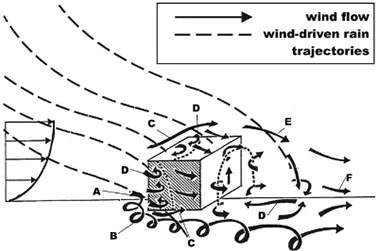
Figure after [Blocken et al., 2004]16
Due to the specific characteristics of the flow near a building, the path of raindrops is altered, resulting in non-uniform wetting of the facade. Indeed, when the wind approaches a building, a disturbance is generated, and a specific flow pattern develops around it, including a frontal vortex (A), corner currents (B), separation at building corners (C), recirculation zones (D), shear layers (E), and a far wake (F).
Rain intensity vectors
The combined occurrence of wind and rain gives rise to an oblique rain intensity vector.
This oblique vector is sometimes referred to as “driving rain” or more generally, “wind-driven rain” (WDR). Thus, the term “wind-driven rain intensity” generally refers to the oblique rain vector (\(R\)). This vector is defined for each raindrop diameter. Its magnitude is equal to the fraction of rain intensity for that specific diameter, and its direction is determined by the trajectory of the wind-driven rain.
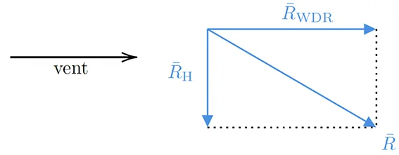
Figure after [Blocken et al., 2004]16
However, to address the interaction between rain and the vertical facades of buildings, we refer to the decomposition illustrated in Figure 6. The term “wind-driven rain intensity” (WD) corresponds to the horizontal component of the oblique rain intensity vector (\(R_{\text{WDR}}\)), which results in a flow of rain through a vertical plane 7. The other, vertical component of the oblique rain intensity vector (\(R_{\text{H}}\)), which causes a flow of rain through a horizontal plane, is called “horizontal rain intensity.” This latter vector \(R_{\text{H}}\) corresponds to the regular intensity of precipitation \(\left|| R_{\text{H}} \right|| = r_{\text{h}}\), as measured by meteorological stations.
[Hoppestad, 1955]17 proposes the following relationship to relate wind speed $U$ to rain intensity $r_{\text{h}}$.
$$ r_{\text{wdr}}= r_{\text{h}} \frac{U}{V_{\text{t}}(\phi)} \text{~~~~~(4)} $$Where $r_{\text{wdr}}= \left|| R_{\text{WDR}} \right||$ can be understood as the proportion of rain passing through a vertical plane [l/m²/h].
Wind-Driven Rain Load
There are several quantities used to describe the wind-driven rain load on facades. Among these, the most commonly used ones are the specific catching ratio \(\eta_{\phi}\) (related to the raindrop diameter) and the catching ratio \(\eta\) (related to the entire raindrop diameter spectrum) [Blocken et al., 2004]16.
These catching ratios are defined at a specific time ($t$) as the ratio between the wind-driven rain intensity (\(r_{\text{wdr}}\)) and the meteorological rain (horizontal) intensity (\(r_{\text{h}}\)) for a raindrop diameter (\(\phi\)) where the entire spectrum is considered.
$$ \eta_\phi\left(\phi,t\right) = \frac{r_{\text{wdr}}\left(\phi,t\right)}{r_{\text{h}}\left(\phi,t\right)} \text{~~~~~(5)} $$$$ \eta\left(t\right) = \frac{r_{\text{wdr}}\left(t\right)}{r_{\text{h}}\left(t\right)} $$In practice, these ratios will be calculated or measured for discrete time intervals. In that case, they are written as follows:
$$ \eta_\phi\left(\phi,t_j\right) = \frac{\int_{t_j}^{t_j+\Delta t} r_{\text{wdr}} \left(\phi,t\right) dt}{\int_{t_j}^{t_j+\Delta t} r_{\text{h}} \left(\phi,t\right) dt} \text{~~~~~(6)} $$$$ \eta\left(t_j\right) = \frac{\int_{t_j}^{t_j+\Delta t} r_{\text{wdr}} \left(t\right) dt}{\int_{t_j}^{t_j+\Delta t} r_{\text{h}} \left(t\right) dt \frac{U}{V_{\text{t}}(\phi)}} $$Catching ratios are complex functions of space and time. Six fundamental parameters influence them, including the building’s geometry, including the environmental topology (i), the position on the building’s facade (ii), wind speed (iii), wind direction (iv), horizontal precipitation intensity (v), and the distribution of raindrop sizes (vi). Although often overlooked, turbulent dispersion of raindrops could also be considered as an additional parameter.
Semi-empirical methods
The classic meteorological data measured at weather stations include wind direction and speed, as well as rain intensity ($r_{\text{h}}$).
Researchers have sought to calculate the exposure of building facades to wind-driven rain based on this meteorological data. They have established semi-empirical relationships through empirical observations, which link wind-driven rain intensity (\(WD\)) with wind speed and measured rain intensity. Existing calculation methods largely stem from two approaches initiated by [Hoppestad, 1955]17: the WD rain index and the WD rain formula.
Rain index $WD$
The wind-driven rain index is calculated as the product of wind speed and the measured rain intensity (\(r_{\text{h}}\)). This index is approximately proportional to the wind-driven rain intensity (\(r_{\text{wdr}}\)). In its original form, it is a qualitative measure of a location’s exposure to unobstructed wind-driven rain intensity, meaning it is away from any obstacles.
At its creation, the wind-driven rain index had several shortcomings [Blocken et al., 2004]16: it was based on annual average values, making it a long-duration index (i). As such, it should be associated with long-term events such as moisture accumulation in porous materials but not short-term events such as penetration through windows (ii). The WDR index relates to free WDR and therefore does not take into account local phenomena induced by topography and the building (iii).
New developments and improvements over the past few decades have transformed the index into a quantitative measure of a building wall’s exposure to wind-driven rain. To achieve this, hourly wind and rain data were introduced into the index calculations (i). A second index was added alongside the annual average index to represent short-duration WDR events (ii). Empirical factors were included to account for the effects of terrain roughness, local topography, obstructions, and building geometry (iii).
Rain formula $WD$
The WD rain relation is a formula that links wind-driven rain intensity to the usual variables, which are wind speed, wind direction, and precipitation intensity \(r_{\text{h}}\), by introducing a WD rain coefficient. Based on Equation (4), which provides an estimate of unobstructed wind-driven rain intensity, [Lacy, 1965]18 proposes a value for the WD rain coefficient by using the median size of raindrops. The relation (4) then becomes \(r_{\text{wdr}} = 0.222Ur_{\text{h}}\). This WD rain coefficient is subsequently refined and takes into account the effects of wind orientation on the facade. The final relation is expressed as:
$$ r_{\text{wdr}} = \alpha U r_{\text{h}} \cos \left(\theta\right) \text{~~~~~(7)} $$Where $\theta$ is the angle between the wind direction and the wall’s normal, and \(\alpha\) is the WD rain coefficient.
The main challenge in using Equation (7) is obtaining a reliable WD rain coefficient. It depends on a large number of parameters and varies for each situation and wind-driven rain scenario considered. A WD rain coefficient can be obtained through short-term or long-term measurements. In the first case, you get a WD rain coefficient that is representative only of the measured period, while in the second case, you obtain a coefficient that is representative only of the average of the measured situations.
PrEN 13013-3 method
The European standard project PrEN 13013-3 envisions a procedure that relies on both the WD rain index and the WD rain relation. It inherently uses an adapted WD rain coefficient, which is determined as the product of the free WD rain coefficient (0.222 s/m) by four correction factors determined empirically. These four correction factors are \(R\) (terrain roughness factor), \(T\) (topography factor), \(O\) (obstruction factor), and \(W\) (wall factor).
This correction yields the coefficient \(\alpha\) in Equation (7). This correction makes the formula better than the traditional practice of using the WD rain relation with a single WD rain coefficient. The latter, in fact, does not account for variations in the WD rain coefficient with the building’s geometry and the position on the building’s facade.
However, the standard project also has several drawbacks: it can only be applied to specific building configurations (i). The wall factors in the charts provide limited information about spatial variation across the facade (ii). The WD rain coefficient \(\alpha\) is assumed to be constant for a fixed position on the building, meaning it’s constant over time (iii). It is assumed that the factor \(\cos(θ)\) is sufficient to account for the effect of wind direction variation (iv).
Numerical modeling
Lagrangian ou Eulerian model
The most common method in the literature for modeling the effects of wind-driven rain on building facades is based on the extension of Choi’s steady-state approach [Choi, 1993]19 [Choi, 1994]20 into the time domain by [Blocken et al., 2007a]21 [Blocken et al., 2007b]22. In this approach, the rain phase is resolved through a Lagrangian modeling of raindrops that is unidirectionally coupled with the wind, with the effect of raindrops on the airflow being ignored. This method consists of five steps:
- The wind configuration in steady-state around the building is calculated using 3D RANS turbulence models in steady-state.
- Raindrop trajectories are obtained by injecting particles of different sizes into the calculated airflow.
- The specific capture rate for each raindrop size is determined based on the calculated trajectories.
- The overall capture rate is calculated using the specific capture rate and the horizontal distribution of raindrop sizes.
- Experimental data for wind speed, wind direction, and rain intensity are combined with the capture rates to obtain spatial and temporal distributions of wind-driven rain on the building facades.
Steps (2) and (3) involve a lengthy iterative trial-and-error process to find appropriate injection positions for raindrops so that they cover the entire surface of the studied facade. It is important to note that this procedure must be repeated for each combination of: raindrop size (i), reference wind speed (ii), and reference wind direction to establish a comprehensive table of capture rates for each facade position (iii).
The use of a multiphase Eulerian model for wind-driven rain calculations provides a faster procedure, even for a domain consisting of a single building [Kubilay et al., 2013]23.
In multiphase Eulerian models, the rain phase and the wind phase are considered as continuous mediums. Each raindrop size class is treated as a different phase because each group of similar-sized raindrops will interact with the wind field in a similar way. It is then necessary to impose a boundary condition for each raindrop size class without having to define an injection plane to position correctly. Finally, similar to what is done in the Lagrangian approach, the overall capture rate is calculated by summing the specific capture rates for each phase.
Multiphase Eulerian model equations
The Multiphase Eulerian Model described below is the one developed by [Kubilay et al., 2013]23 and [Kubilay et al., 2015]24 and is available as an open-source model on [Carmeliet’s website]25.
Wind modeling
The authors of [Kubilay et al., 2013]23 propose modeling wind flows using a 3D RANS model with a \(k-\varepsilon\) turbulence model [Markatos, 1986]26 in steady-state. The equations of the model used by [Kubilay et al., 2013]23 are as follows:
$$ \frac{\partial u_j}{\partial x_j} =0 $$$$ \frac{\partial \rho_{\text{a}} u_i}{\partial t} + \frac{\partial\left(\rho_{\text{a}} u_i u_j\right)}{\delta x_j} = - \frac{\partial p}{\partial x_i} + \frac{\partial \tau_{ij}}{\delta x_j} $$$$ \frac{\partial \rho_{\text{a}} k}{\partial t} + \frac{\partial\left(\rho_{\text{a}} k\, u_j\right)}{\partial x_j} = \frac{\partial }{\partial x_j} \left[\left(\mu+\frac{\mu_{\text{t}}}{\sigma_k}\right)\frac{\partial k}{\partial x_j}\right] + G_k - \rho_{\text{a}} \, \varepsilon $$$$ \frac{\partial \rho_{\text{a}} \varepsilon}{\partial t} + \frac{\partial\left(\rho_{\text{a}} \varepsilon\, u_j\right)}{\partial x_j} = \frac{\partial }{\partial x_j} \left[\left(\mu+\frac{\mu_{\text{t}}}{\sigma_\varepsilon}\right)\frac{\partial \varepsilon}{\partial x_j}\right]+ C_{1_\varepsilon}\frac{\varepsilon}{k}G_k-C_{2_\varepsilon}\rho_{\text{a}}\frac{\varepsilon^2}{k} $$$$ \mu_{\text{t}}=C_\mu \rho_{\text{a}} \frac{k^2}{\varepsilon} $$Where $\rho_{\text{a}}$ represents the air density, $p$ is the pressure, $\tau_{ij}$ is the Reynolds stress tensor, $k$ is the turbulent kinetic energy, $\varepsilon$ is the turbulent dissipation, $\mu$ is the dynamic viscosity of air, $\mu_{\text{t}}$ is the turbulent dynamic viscosity of air, $\sigma_k$ the turbulent Prandtl number for $k$, $\sigma_\varepsilon$ the turbulent Prandtl number for $\varepsilon$, $G_k$ the generation of turbulent kinetic energy due to mean velocity gradients.
The following values of model constants are used by [Kubilay et al., 2013]23: $C_{1_\varepsilon}=1.44$, $C_{2_\varepsilon}=1.92$, $C_{\mu}=0.09$, $\sigma_k=1.0$, $\sigma_\varepsilon=1.3$.
In the $k-\varepsilon$ model, the Reynolds stress tensor is modeled using turbulent viscosity,\(\mu_{\text{t}}\), assumed to be an isotropic quantity. Therefore, errors increase in regions where the effects of anisotropic turbulence become relatively significant.
The volumetric ratio of rain in the air is less than \(1 \times 10^{-4}\). Therefore, it is reasonable to consider a unidirectional coupling between the wind and$ raindrops [Elghobashi, 1994]27.
Transport of Raindrops
The equations of mass and momentum conservation for raindrops are solved by considering each raindrop size class as a different phase.
The equations that govern each rain phase \(k\) according to [Kubilay et al., 2015]24 are as follows:
$$ \frac{\delta \rho_{\text{w}}\alpha_k}{\delta t}+\frac{\delta\left(\rho_{\text{w}}\alpha_k u_{kj}\right)}{\delta x_j}=0 $$$$ \frac{\delta \rho_{\text{w}}\alpha_k u_{ki}}{\delta t}+\frac{\delta\left(\rho_{\text{w}}\alpha_k u_{ki} u_{kj}\right)}{\delta x_j} = \rho_{\text{w}} \alpha_k g + \rho_{\text{w}} \alpha_k \frac{3 \mu}{\rho_{\text{w}} \phi^2} \frac{C_d \mathrm{Re}\_{\text{p}\_\text{r}}}{4} \left(u_i-u_{ki}\right) $$Where \(\phi\) is the diameter of the raindrops, \(\alpha_k\) is the volumetric fraction of the \(k\)-th rain phase, \(u_{ki}\) is the \(i\)-th component of the velocity vector of the \(k\)-th rain phase, \(u_i\) is the wind velocity component, \(\rho_{\text{w}}\) is the density of raindrops, \(g\) is the gravitational acceleration, \(C_{\text{d}}\) is the drag coefficient. \(\mathrm{Re}_{\text{p}_\text{r}}\) represents the relative Reynolds number calculated as follows:
$$ \mathrm{Re}\_{\text{p}\_\text{r}}=\frac{\rho\_{\text{a}} \phi}{\mu} \left||\bar{u}-\bar{u}\_k\right|| $$Where $\bar{u}$ is the wind velocity vector $\bar{u}\_k$ is the velocity vector of the $k$-th rain phase.
The effects of turbulent dispersion of raindrops can be introduced into the transport equation by adding a term that depends on the velocity fluctuations \(u_{ki}^\prime\). This results in the following equation:
$$ \frac{\delta \rho_{\text{w}}\alpha_k u_{ki}}{\delta t}+\frac{\delta\left(\rho_{\text{w}}\alpha_k u_{ki} u_{kj}\right)}{\delta x_j} +\frac{\delta\left(\rho_{\text{w}}\alpha_k u^\prime_{ki} u^\prime_{kj}\right)}{\delta x_j}= \rho_{\text{w}} \alpha_k g + \rho_{\text{w}} \alpha_k \frac{3 \mu}{\rho_{\text{w}} \phi^2} \frac{C_d \mathrm{Re}\_{\text{p}\_\text{r}}}{4} \left(u_i-u_{ki}\right) $$The authors of [Kubilay et al., 2015]24 suggest introducing a new coefficient $C_{\text{t}}$ such that:
$$ C_{\text{t}}^2 = \frac{u^\prime_{ji} u^\prime_{kj}}{u^\prime_i u^\prime_j} = \frac{1}{1+\frac{\tau_{\text{p}}}{\tau_{\text{fl}}}} $$Where $\tau_{\text{p}}$ is the relaxation time of the particles: the time it takes for the particle’s acceleration to respond to the relative velocity between the particle and the carrying fluid. \(\tau_{\text{fl}}\) is the fluid timescale: the characteristic lifespan of large eddies. For the smallest raindrops, \(C_{\text{t}}\) tends toward 1. In this case, raindrops are more influenced by wind velocity fluctuations.
Catching Ratios
The specific and overall catching ratios representing the wind-driven rain load on the facades are numerically evaluated from the following expressions:
$$ \eta_k\left(\phi_k\right) = \frac{\alpha_k \left|| \bar{V}\_k(\phi_k) \right|| }{r_{\text{h}} f_{\text{h}}\left(r_{\text{h}}, \phi_k\right)} $$$$ \eta=\int_k f_{\text{h}}(\phi_k) \eta_k (\phi_k)d \phi_k $$Where $r_{\text{h}}$ is the rain intensity, $f_{\text{h}}\left(r_{\text{h}}, \phi\right)$ is the drop size distribution function with the cumulative probability law given by equation (3), and $\left||\bar{V}\_k(\phi)\right||$ is the norm of the velocity vector of the \(k\)-th phase projected onto the normal to the studied facade.
Boundary Conditions
Wind
At the domain inlet, the average wind velocity is calculated using the classical formula for the atmospheric boundary layer:
$$ u(z) = \frac{u^{\*}}{\kappa}\ln\left(\frac{z+z_0}{z_0}\right) $$With \(u(z)\) being the wind velocity at height \(z\), \u^{*}\) representing the friction velocity of the atmospheric boundary layer, \(\kappa\) is the von Karman constant (0.42 in this case), and \(z_0\) is the aerodynamic roughness height.
The turbulent variables $k$ and $\varepsilon$ can be taken from the following equations.
$$ k = \left(I u\right) ^2 $$$$ \varepsilon = \frac{u^{\*3}}{k \left(z+z_0\right)} $$Where \(I\) is the turbulence intensity.
Finally, wall functions must be properly defined for the walls. For this, one can refer to classical wall functions such as those from [Launder et al., 1983]28. These wall functions may be augmented with a roughness model based on the nature of the surfaces considered in the study
Rain
The volumetric fraction of the $\phi$ phase of the rain, $\alpha_\phi$, can be obtained through the following equation:
$$ \alpha_\phi=\frac{r_{\text{h}} \, f(r_{\text{h}}, \phi)}{V_{\text{t}}(\phi)} $$Where $V_{\text{t}}(\phi)$ is the terminal velocity of a raindrop with diameter $\phi$, as approximated by equation (2) and $f(r_{\text{h}}, \phi)$ can be calculated by differentiating equation (3):
$$ f(r_{\text{h}}, \phi)=\frac{n}{A r_{\text{h}}^p} \exp\left[-\left(\frac{\phi}{A r_{\text{h}}^p}\right)^n\right] \left(\frac{\phi}{A r_{\text{h}}^p}\right)^{\left(n-1\right)} $$Where $A$, $p$ et $n$ are the constans in the [Best, 1950]14 model define earlier.
The value of the volumetric ratio for each rain phase, \(\alpha_\phi\), is imposed at the domain inlet and upper boundaries. For the velocity of the rain phase, it is assumed that the domain boundaries are far enough from the buildings so that the flow is not disturbed.
At the inlet of the domain, the vertical component of the rain phase’s velocity corresponds to the terminal velocity \(V_{\text{t}}(\phi)\) for that phase. The horizontal components of the rain phase’s velocity at the inlet of the domain are set equal to the components of the wind velocity.
The boundary conditions for the rain phases at the building, walls, and ground are such that the normal gradient $\partial\alpha_\phi/\partial \bar{n}$ is set to zero when the normal wind velocity vector is directed outward from the domain. On the contrary, when the normal wind velocity vector is directed inward into the domain, [Kubilay et al., 2013]23 set $\alpha_\phi=0$.
Such boundary conditions do not account for the interaction between raindrops and walls. Raindrops therefore exit the domain as soon as they touch a wall, so that even in the presence of recirculation zones, no flow of rain entering the domain is modeled.
J. M. Péerez-Bella, J. Dominguez-Hernandez, B. Rodriguez-Soria, J. J. del Coz-Diaz, and E. Cano-Suñen. Combined use of wind-driven rain and wind pressure to define water penetration risk into building facades: the spanish case. Building and Environment, 64:46-56, 2013. DOI ↩︎
L. Franke, I. Schumann, R. Van Hees, L. Van der Klugt, S. Naldini, K. Van Balen, and J. Mateus. Damage atlas, classification and analysis of damage patterns found in brick masonry. 1995. ↩︎
X. Zhou, J. Carmeliet, and D. Derome. Assessment of risk of freeze-thaw damage in internally insulated masonry in a changing climate. Building and Environment,page 106773, 2020. Lien PDF ↩︎
S. J. Granneman, B. Lubelli, and R. P. van Hees. Mitigating salt damage in building materials by the use of crystallization modifers-a review and outlook. Journal of Cultural Heritage, 40:183-194, 2019. DOI ↩︎
P. J. Annila, M. Hellemaa, T. A. Pakkala, J. Lahdensivu, J. Suonketo, and M. Pentti. Extent of moisture and mould damage in structures of public buildings. Case studies in construction materials, 6:103-108, 2017. Lien PDF ↩︎
J. Slusarek and M. Lupie-zowiec. Analysis of the in uence of soil moisture on the stability of a building based on a slope. Engineering Failure Analysis, page 104534, 2020. DOI ↩︎
B. Blocken, D. Derome, and J. Carmeliet. Rainwater runooff from building facades: A review. Building and Environment, 60:339-361, 2013. Lien PDF ↩︎ ↩︎
R. B. White. The changing appearance of buildings. 1967. ↩︎
K. V. Beard, V. Bringi, and M. Thurai. A new understanding of raindrop shape. Atmospheric research, 97(4):396-415, 2010. DOI ↩︎
R. Gunn and G. D. Kinzer. The terminal velocity of fall for water droplets in stagnant air. Journal of Me- teorology, 6(4):243-248, 1949. Lien PDF ↩︎
N. Dingle and Y. Lee. Terminal fallspeeds of raindrops. Journal of applied meteorology, 11(5):877-879, 1972. DOI ↩︎
J. O. Laws and D. A. Parsons. The relation of raindropsize to intensity. Eos, Transactions American Geophys- ical Union, 24(2):452-460, 1943. DOI ↩︎
J. S. Marshall and W. M. K. Palmer. The distribution of raindrops with size. Journal of meteorology, 5(4):165- 166, 1948. DOI ↩︎
A. Best. The size distribution of raindrops. Quarterly Journal of the Royal Meteorological Society, 76(327):16-36, 1950. DOI ↩︎ ↩︎ ↩︎ ↩︎
M. Fujiwara. Raindrop size distributions with rainfall types and weather conditions. Technical report, Illinois State Water Survey, 1961. Lien PDF ↩︎
B. Blocken and J. Carmeliet. A review of wind-driven rain research in building science. Journal of wind en- gineering and industrial aerodynamics, 92(13):1079-1130, 2004. Lien PDF ↩︎ ↩︎ ↩︎ ↩︎
S. Hoppestad. Driving rain in norway. Norwegian Build- ing Research, 1955. DOI ↩︎ ↩︎
R. E. Lacy. Driving rain maps and the onslaught of rain on buildings. In Proc. of CIB/RILEM Symposium on Moisture Problems in Buildings, Helsinki, 1965, 1965. ↩︎
E. Choi. Simulation of wind-driven-rain around a building. In Computational Wind Engineering 1, pages 721- 729. Elsevier, 1993. Lien PDF ↩︎
E. Choi. Determination of wind-driven-rain intensity on building faces. Journal of Wind Engineering and Industrial Aerodynamics, 51(1):55-69, 1994. DOI ↩︎
B. Blocken and J. Carmeliet. On the errors associated with the use of hourly data in wind-driven rain calculations on building facades. Atmospheric Environment, 41(11):2335-2343, 2007. Lien PDF ↩︎
B. Blocken and J. Carmeliet. Validation of cfd simulations of wind-driven rain on a low-rise building facade. Building and Environment, 42(7):2530-2548, 2007. Lien PDF ↩︎
A. Kubilay, D. Derome, B. Blocken, and J. Carmeliet. Cfd simulation and validation of wind-driven rain on a building facade with an eulerian multiphase model. Building and environment, 61:69-81, 2013. Lien PDF ↩︎ ↩︎ ↩︎ ↩︎ ↩︎ ↩︎
A. Kubilay, D. Derome, B. Blocken, and J. Carmeliet. Wind-driven rain on two parallel wide buildings: feld measurements and cfd simulations. Journal of Wind Engineering and Industrial Aerodynamics, 146:11-28, 2015. Lien article ↩︎ ↩︎ ↩︎
J. Carmeliet. Wind-driven rain solver for openfoam. https://carmeliet.ethz.ch/research/downloads/ winddrivenrainfoam.html. Lien PDF ↩︎
N. Markatos. The mathematical modelling of turbulent flows. Applied Mathematical Modelling, 10(3):190-220, 1986. DOI ↩︎
S. Elghobashi. On predicting particle-laden turbulent flows. Applied scientifc research, 52(4):309-329, 1994. Lien PDF ↩︎
B. E. Launder and D. B. Spalding. The numerical computation of turbulent flows. In Numerical prediction of flow, heat transfer, turbulence and combustion, pages 96-116. Elsevier, 1983. Lien PDF ↩︎