 L'hypercube
Computation of the Mean Radiant Temperature
Definition
The Mean Radiant Temperature \(T_{\text{r}}\) is defined as the uniform temperature of an enclosure in which the radiant heat transfer is equal to radiant heat transfer in the real, non-uniform enclosure. Indeed, indoor and outdoor environments can be rather complex, integrating solar fluxes \(\varphi\) or different surface temperatures. The mean radiant temperature hence combines all radiant contributions in a unique indicator.
The mathematical expression is as follows:
$$ \sigma \epsilon S T_{\text{r}}^4 = \alpha S \varphi + \sigma \epsilon \sum_{i=1}^{n} S_i F_i T_i^4 $$where \(F_i\) are the View Factors between surfaces at a temperature \(T_i\) and the studied body.
In the following sections, we will first discuss solar contribution to radiant temperature and then the contribution of infrared radiation.
Solar Contribution
A blunt method of calculating the short-wavelength component is to apply the projection factor method, which considers that the direct normal flux \(\varphi^\perp\) is applied on the human body with a projection factor taking into account the cylindrical nature of the human body:
$$ \varphi = \alpha \varphi^\perp f_{\text{p}}(h) $$where the projection factor depends on the solar height: \( f_{\text{p}}(h) = 0.233 \cos(h) + 0.067\).
This simple method can be refined by considering the solar contribution as divided into a diffuse part, \(\varphi_{\text{d}}\), and a direct one, \(\varphi_{\text{b}}\), treated separately due to their nature, as described in the following sections.
Direct flux
The direct flux arriving on a cylindrical individual can be computed analytically from the direct lux on a horizontal plane \(\varphi_{\text{b}}^h\), knowing the solar altitude angle \(h\) and the angle of incidence \(i\):
$$ \varphi_{\text{b}} = \varphi_{\text{b}}^{\text{h}} \times \frac{\cos(i)}{\sin(h)} $$The flux received on the cylinder is calculated analytically from the following geometrical configuration and the angle of incidence \(\theta\) with respect to the normal to the cylinder surface.
This translates into the following integral, the result of which is the projected surface rthogonal to sun rays, which by the nature of the cylinder is always azimuthal (i.e. in the axis of the sun’s rays):
$$ \phi_{\text{b}} = \int_{-\frac{\pi}{2}}^{\frac{\pi}{2}} \varphi_{\text{b}} \cos(\theta) r H d\theta = 2 \varphi_{\text{b}} r H = S_{\text{p}} \varphi_{\text{b}} $$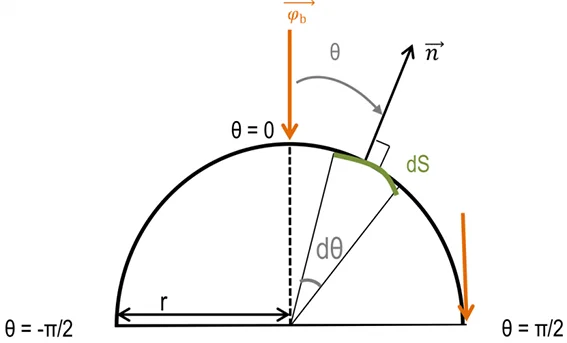
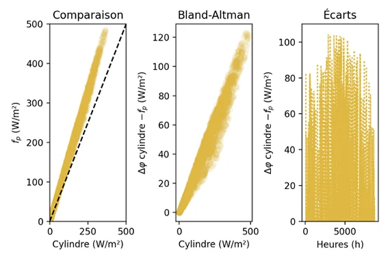
Note: In practice, using this method provides similar received solar flux values as the \(f_{\text{p}}\) method for direct flux (see [Walther & Hamdani]1)
The value of direct solar flux calculated by the \(f_{\text{p}}\) method is however slightly higher, as shown in the model comparison below.
Diffuse flux
Perez2’ diffuse solar flux model is used ( more details ), considering the circumsolar, horizon brightening and isotropic dome contributions, as per the following figure:
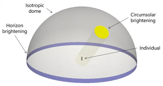
In the following, we hypothesize that the dome contribution (\(L\)) and horizon contribution (\(K_2\)) are isotropic on the cylinder, and that the circumsolar, anisotropic, contribution (\(K_1\)) behaves as if it were specular, lighting “directly” the scene (see sketch below):
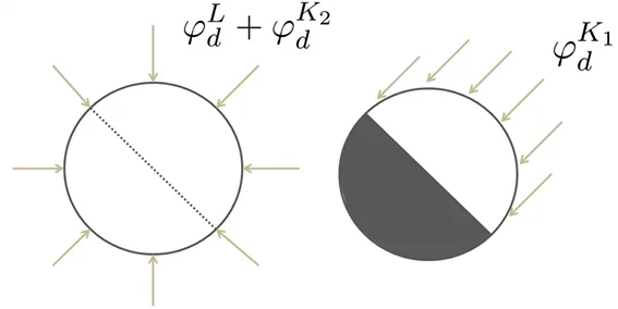
The total diffuse flux received is hence computed as:
$$ \phi_{\text{d}} = 2 r H \varphi_{\text{d}}^{K_1} + 2 \pi r H \times (\varphi_{\text{d}}^L +\varphi_{\text{d}}^{K_2} ) = S_{\text{p}} \varphi_{\text{d}}^{K_1} + S_{\text{c}} (\varphi_{\text{d}}^L +\varphi_{\text{d}}^{K_2} ) $$Numerical verification
The total solar flux received is then \(\phi = S_{\text{p}}\varphi_{\text{b}} + \phi_{\text{d}}\) in [W].
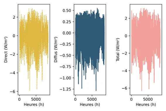
Comparing the analytical model of the cylinder presented above with those of a discrete, 12 faced cylinder
(using the package pvlib
), we obtain following results,
showing a good agreement between both models.
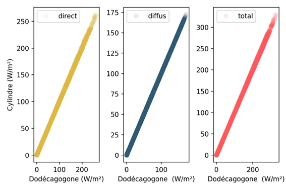
The discrepancies between models are given below and present an RMSE inferior to 0.76 [W/m²] for the three solar fluxes, which demonstrates the validity of the approach.
Results for three summer days
An example of application of the method described hereinabove is plotted for three summer days on the figure below. The same orders of magnitude as in the experimental literature are found ([Kantòr et al. 2018]3, [Park et al. 2018]4) as well as the “daytime relapse” phenomenon identified by [Kantòr et al. 2013]5. The comparison with the so-called “6-directions” method (also described here ) yields similar results.
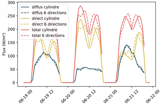
The analogy of the results with those obtained by the projection factor method, derived by Fanger for an ndividual, leads to the conclusion that the cylindrical integral method is suitable for modelling the flux received by humans
The results obtained are of the same order of magnitude as those of the “6-directions” method, whose pitfalls were presented in [Kantòr et al. 2018]3.
The advantage of the presented method is that it requires only the direct and diffuse horizontal fluxes, as well as the solar height, which are usually present in meteorological files or easily determined with freely available tools.
The method could be extended to an ellipse whose analytical formula is known in order to approximate other projection factor configurations proposed in the literature.
Infrared contribution
The calculation of the long wave contribution is made possible by determining the view factors between
facing walls. For this purpose, the pyViewFactor
code is used,
as described in our paper from IBPSA France 2022 conference
6.
Principle
Taking a geometrical representation of an individual as an octagon, one wishes to calculate the contribution of different walls in a room. The radiation view factor is defined as the ratio of the fluxes received by a wall (or a set of walls) to the total flux “outgoing” from the emitting wall. Thus it can be calculated by summing the fluxes between the \(n\) cells of a discretized wall and the 9 faces of a the “individual” (8 faces of the octagon plus the cap):
$$ F_{\text{p}} = \frac{ \sigma \epsilon \sum_{j=1}^{9} \sum_{i=1}^{n} S_i F_{ij} T_{\text{p}}^4 }{ \sigma \epsilon S T_{\text{p}}^4} = \frac{ \sum_{j=1}^{9} \sum_{i=1}^{n} S_i F_{ij}}{S} $$View Factors of the walls to an individual in the centre of a room
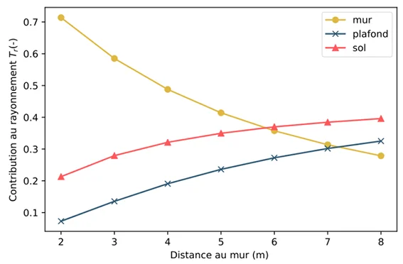
An application of this method is the calculation of the contribution of each wall to the radiation balance of an individual located in the centre of a room, as shown in the following figure.
The calculation is carried out for different room lengths: the results are given in the figure below. As the individual is positioned in the centre of the zone, it can be seen that the contribution of the vertical walls decreases significantly with the size of the room. After about ~6 metres, it can be seen that the contributions f the different walls are roughly equivalent: one third for the floor, one third for the ceiling and one third or the four walls of the room.
View factors of walls depending on the position in a room
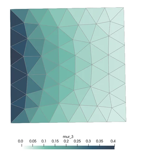
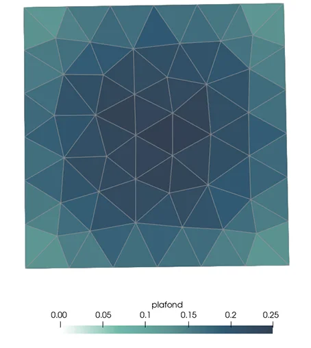
We are now interested in the influence of the various walls with regards to the individual’s position on the floor. The same calculation is carried out for each cell of the floor mesh, by successively repositioning the individual-octagon at each cell center.
The following maps are obtained, giving the view factor of each wall towards the individual, depending on its position in the room:
Spatial Mean Radiant Temperature
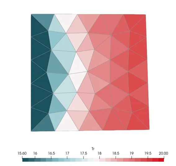
This makes it possible to calculate the radiant temperature in the room as a function of the individual’s position. To determine this, the equation is solved for \(T_{\text{r}}\) giving the radiant temperature of the room walls that would cause the same radiative exchange as the existing walls, with their respective areas and view factors:
$$ \sigma \epsilon \sum_{i=1}^{n} S_i F_{i} T_{\text{r}}^4 = \sigma \epsilon \sum_{i=1}^{n} S_i F_i T_i^4 $$Let
$$ T_{\text{r}} = \sqrt[4] { \frac{ \sum_{i=1}^{n} S_i F_i T_i^4 }{\sum_{i=1}^{n} S_i F_{i} } } $$Performing the calculation on a cubic room where the walls are at 20°C, except for one wall at 0°C, we obtain the following result, which shows a difference of ~6 K in radiant temperature difference.
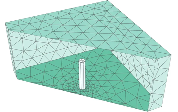
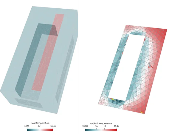
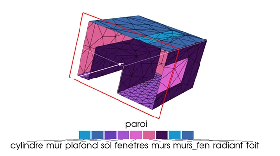
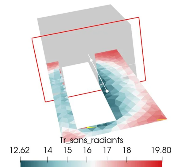
For a more complex configuration, e.g. a train maintenance facility, including windows, radiant panels and a train at the outside temperature, the following results are obtained:
View factor diagrams between a person and a wall
In order to update and make more readable Fanger’s work presenting the form factor between an individual and
different walls (see the example below giving the form factor with a ceiling), we’re going to use the
pyViewFactor
package.
The geometry of the individual is taken from the doorman
example from PyVista
. In order to simplify the calculations, a
version with fewer cells has been created using the decimate filter. As an example, the image below shows the
form factor between the facets making up the individual and the ground.
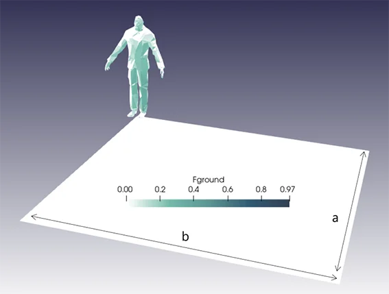
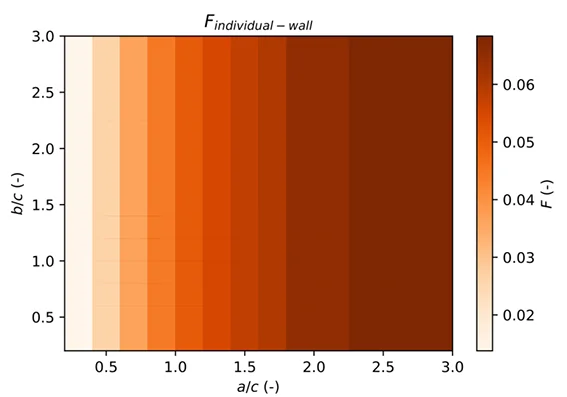
The resulting abacus is shown below:
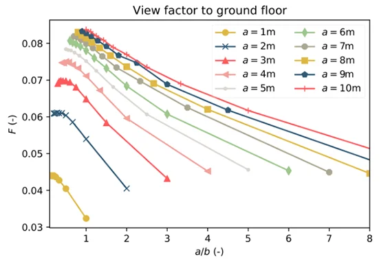
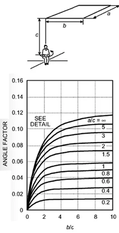
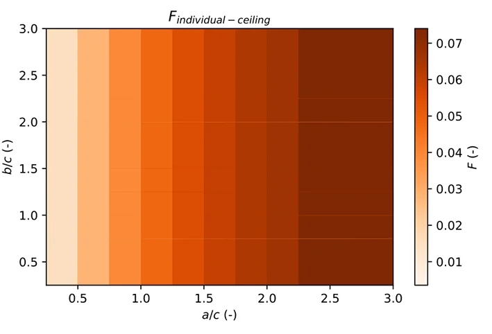
The abacus of the form factor of an individual towards a ceiling of dimensions \(a\), \(b\) = length, width and height \(c\) is shown below.
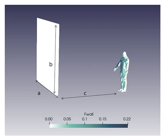
The view factor between an individual and a wall, as shown in the figure below, is given in the graph below (the orientation of the individual has a marginal influence on the result).
Walther, E., Hamdani, E.M. 2018, Calcul trigonométrique du flux solaire reçu par un individu, IPBSA 2018 PDF link ↩︎
Perez, R., Seals, R., & Michalsky, J. (1993). All-weather model for sky luminance distribution—preliminary configuration and validation. Solar energy, 50(3), 235-245. PDF link ↩︎
Kántor N., Viktória Gál, C. , Gulyás, A., Unger, J., 2018, The Impact of Façade Orientation and Woody Vegetation on Summertime Heat Stress Patterns in a Central European Square: Comparison of Radiation Measurements and Simulations PDF link ↩︎ ↩︎
Park, S., Tuller, S.E., 2011, Comparison of human radiation exchange models in outdoor areas Theor Appl Climatol 105, 357–370 DOI ↩︎
Kántor, N., Lin, P. T.,Matzarakis, A., 2013 Daytime relapse of the mean radiant temperature based on the six-directional method under unobstructed solar radiation PDF Link ↩︎
Bogdan, M., Walther, E., Alecian, M., Chapon, M., 2022, Calcul des facteurs de forme entre polygones -Application à la thermique urbaine et aux études de confort, IBPSA France, PDF Link ↩︎