 L'hypercube
Comfort modeling
Comfort modelling in semi-open spaces, with variable environmental conditions and potentially transient occupancy, requires a higher level of detail than is generally used in buildings. Conventional steady-state approaches of the PMV type are unsuitable for such environments and a transient model of human metabolism is then used. In the following page, we present a comfort indicator based on such a model, as well as an exploration of the influence of physiological variability.
Introduction
Many approaches have been developed to quantify the level of comfort of individuals in indoor spaces, often for productivity purposes: the first studies in the field consisted in comparing factories’ indoor temperatures with production quality or absenteeism [H.M. Vernon et al., 1936]1.
In peculiar cases, the indoor comfort temperature can be determined by an empirical method. Thus the adaptive approach of [R. De Dear, 2001] used for naturally ventilated buildings gives a linear relationship between comfort temperature and the one-month moving average of the outside temperature, calibrated from thousands of measurements.
In indoor environments, the most commonly used indicator is [Fanger, 1970]2’s Predicted Mean Vote which connects the heat flux (negative or positive) on the individual to the feeling of comfort or discomfort. This link was made possible by combining an equational approach, allowing the heat balance to be established, with a statistical regression on the comfort level of a sample of a few thousand people. However, recent work has shown the limitations of the PMV approach [van Hoof, 2008]3 which is based on a male morphology and causes significant shifts in the comfort range according to gender [Kingma, 2015] .
The equational approach discussed here is the two-node model developed at the J.-B. Pierce Foundation (also called “Pierce’s model”) during the XXst century [Gagge, 1936]4. The purpose was to meet military requirements, including determining the thermal stress resistance of soldiers or fighter pilots under highly variable atmospheric pressures [Nishi, 1977]5. The formulation of the model is relatively simple and consists of representing the human body in the form of two concentric cylinders representing the centre of the body or “core” and the skin layer, surrounded by the clothing (see Fig. 1). In this model, metabolism is a system regulated in temperature by corrective actions (vasomotricity, sweating, perspiration) that evolve over time and according to the surrounding conditions.

Indeed, in outdoor or semi-outdoor environments, rapid variations in ambient conditions make steady-state approaches unsuitable for predicting comfort. This is all the more true when these spaces are occupied temporarily (e.g. outside passageways, very open buildings, stations): the temperature rise time of the metabolism is about one hour in summer and several hours in winter [Hoeppe, 2002]6.
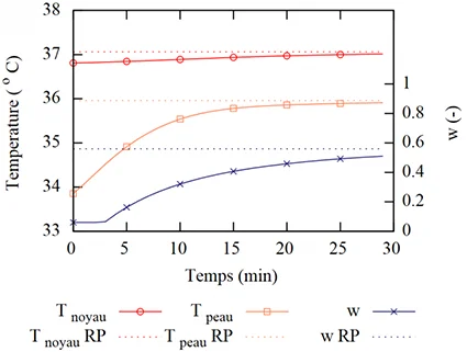
As an illustration, Fig. 2 shows the simulation of body temperatures and skin wetness of an individual with Pierce’s two-node model. From the state of thermal equilibrium, the individual is put in a warm environment with strong solar radiation for thirty minutes. The evolution of body temperatures under transient conditions (solid lines) shows an asymptotic evolution towards the steady state that would be obtained under these conditions (dotted lines). Skin wetness follows a slightly slower dynamic and the steady state is not reached in half an hour of exposure.
The physiological reactions generated by the environment on metabolism via convection, radiation and water exchanges allow to calculate the SET (Standard Effective Temperature). This is the operating temperature of a reference environment that would produce the same skin temperature and skin wetness as the actual environment being studied. This reference environment has a low air velocity, a relative humidity of 50% and the clothing is standardized with respect to the individual’s activity.
The following sections provide a mathematical description of the human body and associated transfers in order to determine the SET from its physiological reactions. The effect of the environment on comfort will then be discussed, and the influence of physiological variability on the dispersion of results will be explored.
Activity and clothing characteristics
In this section, the morphological characteristics of humans and their clothing are described.
Metabolic activity
The metabolism is broken down into so-called “basal” metabolism, which maintains temperature, and activity metabolism, which is linked to the task performed. The term basal metabolic activity, \(M\) [W], expressed as a function of height \(H\) [m], of mass \(m\) [kg] and of age and is calculated using the equation below from [VDI, 2008]7:
$$ M = a \times m^{0.75} \left( 1 + b \times (30.0 - \text{age} ) + c \times \left( \frac{100H}{m^{1/3}} - d \right) \right) $$For both male and female individuals, the constants \(a\), \(b\), \(c\) and \(d\) respectively take the values \(a\)=3.45, \(b\)=0.004, \(c\)=0.01, \(d\)=43, and \(a\)=3.19, \(b\)=0.004, \(c\)=0.018 and \(d\)=42.1.
The surface area of the human body (in m²) is determined from the empirical equation of Dubois which gives a relationship between size \(H\) and mass \(m\):
$$ A = 0.203 \times m^{0.425} \times H^{0.725} $$A typical value for an average individual is \(A \sim\) 1.8 [m²].
The metabolic source term can be computed by two methods:
- either directly in [met] with 1 [met] = 58.2[W/m²] of body surface area. A light office activity generally corresponds to 1 [met],
- or as a combination of basal metabolism and activity metabolism related to the execution of the task, generally in [W] which is converted to [W/m²] using the two previous relationships.
The table below gives some orders of magnitude of the heat released as a function of activity.
| Activity | [W/m²] | [met] |
|---|---|---|
| Rest, lying down | 45 | 0.8 |
| Rest, sittings | 58 | 1 |
| Standing, light office activity | 70 | 1.2 |
| Standing, light activity (lab work) | 95 | 1.6 |
| Medium standing activity (working on a machine) | 115 | 2 |
| Heavy work | 175 | 3 |
Table 1: Metabolism and activity
Clothing properties
Clothing is taken into account via a thermal resistance \(i_{\text{clo}}\) in [clo], such that 1 [clo] = 0.155 [m².K/W] (marked as \( R_\text{cl} \) in this unit).
For example, the value of 1 [clo] corresponds to a shirt, jacket and trousers suit. The table 2 below gives the level of insulation in [clo] for some sets of clothing.
| Clothing | [clo] |
|---|---|
| Light summer clothing | 0.3 |
| Office clothing | 0.7 |
| Indoor winter clothing | 1.0 |
| Outdoor winter clothing | 1.5 |
Table 2: Correspondence between clothing and level of insulation in [clo]
Wearing clothing increases the thermal resistance between the external environment and the skin surface. However, it also increases the surface area exposed to heat transfer: the factor \(f_{\text{clo}}\) is introduced in order to characterize the increase in the heat exchange surface related to the clothing:
$$ f_{\text{cl}} = 1 + k \times i_{\text{clo}} $$In the previous equation, \(k\) = 0.2 if \(i_{\text{clo}}\) < 0.5 and \(k\) = 0.15 else. The surface \(A \times f_{\text{cl}}\) is thus increased by 20% for the wearing of a thermal resistance of 1 [clo].
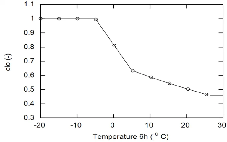
The amount of clothing worn varies according to the weather and individual factors. However, the work of [Schiavon, 2013]8 has shown that the level of individuals’ clothing can be determined from the outside temperature at 6 a.m. on the same day, according to the law shown in Fig. 3.
Equation of human metabolism
In this section, the heat balance on the two nodes of the Pierce model is presented. The calculation of heat and mass transfers to the human body and the regulation of metabolic temperatures are then detailed. Finally, the calculation of the SET will be explained.
Governing equations of Pierce’s model
The two-node model of [Gagge, 1971]9 considers the human body as two concentric cylinders (nucleus and skin) regulated in temperature by several mechanisms: perspiration, sweating, shivering, vasomotricity. Metabolic heat as well as energy dissipated as a result of the activity is represented by a source term. Two balance equations are used to calculate the evolution of the temperature of the skin’s core as a function of radiative, convective and evaporative transfers with the external environment (conduction is neglected for standing posture, the contact surface with the ground being about 2% of that of the body). The figure below gives a representation of the cylindrical model and the heat flux applied:
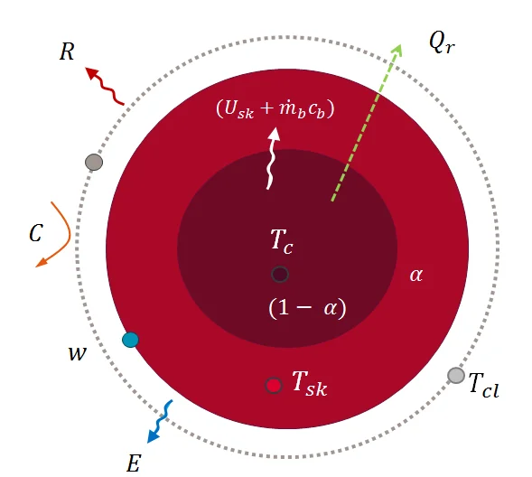
A power balance is then established on the core part, such that the algebraic sum of the metabolic heat \(M\), of the power exchanged with the skin layer (conduction \(U_\text{sk}\) and blood flow \(\dot{m}_{\text{b}} c_{\text{b}}\) and respiratory exchanges \(Q_{\text{r}}\) is equal to the storage of heat in the core \(S_{\text{c}}\) (where the index \(c\) stands for core).
$$ M - \left( U_{\text{sk}} + \dot{m_{\text{b}}} c_{\text{b}} \right) \left( T_{\text{c}} - T_{\text{sk}} \right) - Q_{\text{r}} = S_{\text{c}} $$In the above equation, the term \(M\) stands for metabolic activity in [W/m²], \(U_\text{sk}\) is the thermal conductivity of the tissues between core and skin (such that \(U_\text{sk} =5.28\) [W/(m².K)]). \(\dot{m} c_{\text{b}}\) is the product of the blood mass flow rate \(\dot{m}\) and the heat capacity of blood \(c_{\text{b}} = 4180\) [J/(kg.K)]. \(Q_{\text{r}}\) is the total heat dissipated by breathing (sensible and latent).
At the skin surface, the storage \(S_{\text{sk}}\) (\(sk\) for skin) is the sum of the heat transferred from the core by conduction and by blood flow, of convective heat \(C\), radiant heat \(R\) and evaporative loss \(E\):
$$ \left( U_{\text{sk}} + \dot{m_{\text{b}}} c_{\text{b}} \right) \left( T_{\text{c}} - T_{\text{sk}} \right) - C - R - E = S_{\text{sk}} $$In the above equation, the right hand side represents the energy storage in the skin layer. To the left of equality, the term \(E\) represents the evaporative exchanges on the surface of the skin related to perspiration and sweating. The terms \(C\) and \(R\) respectively represent convective and radiative heat exchange. The equivalent electrical diagram is given below:

Skin mass varies according to the blood flow that swells the external tissues to a greater or lesser extent. The fraction \(\alpha\) of the body mass contained in the outer cylinder of the model is introduced. Variations in skin temperature \(T_\text{sk}\) and core temperature \(T_{\text{c}}\) are then described by following differential equations:
$$ S_{\text{sk}} = \alpha \times \frac{mc_{\text{p}}}{A} \frac{dT_\text{sk}}{dt} $$$$ S_{\text{c}} = (1-\alpha) \times \frac{mc_{\text{p}}}{A} \frac{dT_{\text{c}}}{dt} $$In the second equation, the thermal capacity of the body is \(c_{\text{p}}= 3492\) [J/(kg.K)] and the coefficient \(\alpha\) stands for the fraction of the body mass constituted by the skin, which varies according to the blood flow. Fig. 4 shows the complete model and fluxes.
Note : The percentage of fat mass \(G\) of the human body can be taken into account by weightingthe thermal capacities of the tissues, such that:
$$ c_{\text{p}} = G \times c_{\text{g}} + (1-G) \times c_{\text{b}} $$where respectively \(c_{\text{g}} = 2510\) [J/kg/K] the thermal capacity of fat and \(c_{\text{b}} = 3650\) [J/kg/K] is the one of tissues.
By setting the initial conditions for \(T_\text{sk}\) and \(T_\text{c}\) as the set values \(T_\text{sk}^\text{set}\) and \(T_\text{c}^\text{set}\), it is possible to solve the two temporal differential equations of the two-node model. The model governed by this system thus gives the evolution of body temperatures according to the exchanges with the surrounding environment. The calculation of the various terms presented in the above balance sheets is explained in the following sections.
Respiratory exchanges
The pulmonary ventilation rate is given as a function of metabolic activity in met such that :
$$ \dot{m}_{\text{p}} = 0.3 \times \text{met } \text{ [kg/m$^2$/s]} $$If we convert for a direct calculation with \(M\) in [W/m²] and a flow rate in [kg/s], we get with 1 [met] = 58.2 [W/m²]:
$$ \dot{m}_{\text{p}}= M \times \frac{0.3}{58.2 \times 3600} = M \times 1.432 \times 10^{-6} \text{ [kg/m$^2$/s]} $$The exhaled air temperature is given by the following correlation:
$$ T_\text{exp}= 32.5 + 0.066 \times T_{\text{a}} + 1.99 \times 10 ^{-6} \times p_{\text{a}} $$where \(T_{\text{a}}\) is the air temperature and \(p_{\text{a}}\) is the ambient air vapour pressure in [Pa].
The sensible heat dissipated is then:
$$ C_{\text{resp}} = \dot{m}\_{\text{p}} c_{\text{p}} \left( T\_{\text{exp}} - T\_{\text{a}} \right) $$With \(c_{\text{a}} = 1006\) [J/(kg.K)] for air, we find the well known equation [Thellier, 1989] ,[Fanger, 1970]2:
$$ C_\text{resp} = 1.432 \times 10^{-3} M (T_\text{exp}- T_{\text{a}}) \text{ [W/m$^2$]} $$The above formulation, although widely used, fails to take into account the sensible energy used by the temperature rise of water vapour \(w_{\text{a}}\) [kg/kg] contained in the exhaled air. A rigorous expression of sensible losses by respiration, taking into account the specific heat of the vapour \(c_{\text{v}}\) is the following:
$$ C_{\text{resp}} = \dot{m}_{\text{p}} \times \left( c\_{\text{a}} + w\_{\text{a}}c\_{\text{v}} \right) \times \left( T\_{\text{exp}} - T\_{\text{a}}\right) $$The latent energy dissipated is calculated from the difference in absolute lung moisture \(w_\text{exp}\) and the one of ambiant air \(w_{\text{a}}\):
$$ E\_{\text{resp}} =\dot{m}\_{\text{p}} L_{\text{v}} (w\_{\text{exp}}- w\_{\text{a}}) $$It is more common to work with vapour pressure than with absolute humidity. We therefore convert the previous equation with psychrometric relationships. According to the law of perfect gases, we know that the moisture content of the air depends on atmospheric pressure \(p_\text{atm}\) and the ratio of molar masses of \(M_\text{a}\) and water vapour \(M_{\text{v}}\):
$$ w = \frac{M_{\text{v}}}{M_\text{a}}\times \frac{p_{\text{a}}}{p_\text{atm} - p_{\text{a}}} \simeq 0.622 \times \frac{p_{\text{a}}}{p_\text{atm} - p_{\text{a}}} \text{ [kg/kg]} $$So the equation for the latent energy dissipated becomes:
$$ E\_{\text{resp}} = 0.622 \times \dot{m}\_{\text{p}} L\_{\text{v}} \times \Big (\frac{p\_\text{a}}{p_\text{atm} - p_\text{a}} - \frac{p_\text{v exp}}{p_\text{atm} - p_\text{v exp}} \Big ) \text{ [W/m$^2$]} $$The vapour pressure of the exhaled air is \(p_\text{v exp}\) and at saturated vapour pressure \(p_\text{v exp} = p_\text{vs}(T_\text{exp})\) with the following correlation for the saturated vapour pressure:
$$ p_\text{vs}(T) = 10^{\frac{2.7877 + 7.625 \times T }{241 + T}} $$In general, the above relationship is simplified by considering that the exhaled and ambient vapour pressures (in the order of \(3.10^3\) [Pa]) are small in comparison to atmospheric pressure \(\sim 10^5\) [Pa]. Hence we can write:
$$ p_\text{atm} - p_\text{v} \simeq p_\text{atm} - p_\text{v exp} \simeq p_\text{atm} $$The latent energy dissipated then becomes:
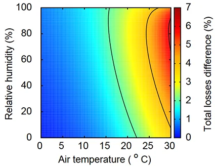
$$ E_\text{resp} \simeq 0.622 \times \frac{\dot{m}\_{\text{p}} L_{\text{v}} }{p\_\text{atm}}(p\_\text{v exp}- p_{\text{a}}) $$$$ E_\text{resp} \simeq 2.14 \times 10^{-5} \times M \times (p_\text{v exp}- p_{\text{a}}) \text{ [W/m$^2$]} $$Neglecting the sensible heat of water vapour and assuming low exhaled pressures in front of atmospheric pressure, has a limited influence: depending on the temperature and humidity conditions considered, the bias introduced is in the order of 2% to 7% between exact and approximate formulations of the sensible and latent losses (the distribution of losses is given in Fig. 6. This deviation may not be negligible insofar as the losses by breathing reach between \(\sim\)25 and 30% of the resting metabolic rate (On this topic, see the [Cain, 1989]10 experiment). Fig. 6, which shows the error between formulations, can be used to determine whether it is necessary to use the exact equations.
Heat Transfer
This section presents the body’s convective and radiative exchanges with the environment.
Convective heat transfer
The natural convection exchange is calculated from the following correlation, weighting the convection coefficient as a function of ambient pressure:
$$ h_{\text{c}}=3\times p_\text{atm}^{0.53}\text{ [W/(m$^2$.K)]} $$When the air velocity \(v\) is known, the following correlation is used, depending on the velocity and atmospheric pressure shown in Fig. 7:
$$ h_{\text{c}} = 8.6 \times (v \times p_\text{atm}\times 10^{-5})^{0.53} \text{ [W/(m$^2$.K)]} $$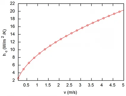
In practice, the maximum value between the two previous equations is taken as the exchange coefficient. The literature is prolific in correlations for the calculation of the convective exchange coefficient on the human being: on this topic we recommand the synthesis made by [Thellier, 1989] .
Radiative heat transfer
Long wave (infra-red) radiant heat transfer between the surface at temperature \(T\) and the surrounding walls at temperature \(T_{\text{r}}\) are modeled via a linearized radiative exchange coefficient \(h_{\text{r}}\) determined as follows:
$$ R = \sigma \varepsilon f (T^4 - T_{\text{r}}^4) $$$$ R = \sigma \varepsilon f (T^2 - T_{\text{r}}^2) (T^2 + T_{\text{r}}^2) $$$$ R =\sigma \varepsilon f (T - T_{\text{r}})(T + T_{\text{r}}) (T^2 + T_{\text{r}}^2) $$Where \(\varepsilon\) is the emissivity of the clothing and \(f\) is a radiation efficiency factor taking into account the fact that some body surfaces do not face the surrounding walls (under the arms, inside the legs).
One then writes out $T_{\text{m}} = (T+T_{\text{r}})/2$, yielding:
$$ R \simeq \sigma \varepsilon f (T - T_{\text{r}}) \times 2 T_{\text{m}} \times 2 T_{\text{m}}^2 $$$$ R\simeq 4 \sigma \varepsilon f T_{\text{m}}^3 \times (T - T_{\text{r}}) = h_{\text{r}} \times (T - T_{\text{r}}) $$Thus we obtain the linearized radiative exchange coefficient \(h_{\text{r}}\):
$$ h_{\text{r}} = 4 \sigma \varepsilon f T_{\text{m}}^3 \text{ [W/(m$^2$.K)] } $$At room temperature, with \(\varepsilon=0.97\) and \(f = 0.72\), we get \(h_{\text{r}} \sim 4.7\) [W/(m².K)].
In outdoor spaces, people are regularly exposed to solar radiation. A simple way of integrating solar fluxes nto the heat balance is to convert them into a rise in the average radiant temperature. The total flux absorbed by the human body is therefore assumed to be equal to that caused by an average radiant temperature \(T_{\text{r}}^*\) greater than \(T_{\text{r}}\).
$$ \alpha f_{p} \varphi_0 = \sigma \varepsilon (T_{\text{r}}^{*4}-T_{\text{r}}^4) $$$$ T_{\text{r}}^{*} = \sqrt[4]{ T_{\text{r}}^4 + \frac{\alpha f_{\text{p}} \varphi_0}{\sigma \varepsilon} } $$Where \(\varphi_0\) is the flux on a surface orthogonal to radiation, \(\alpha \sim 0.7\) is the absorption coefficient of solar radiation, \(f_{\text{p}}\) is a solar radiation projection factor that depends on the solar height \(h\) (a good approximation is given by \(f_{\text{p}} \simeq 0.233 \times \cos(h) +0.067 \) after [Helbig, 2013]11 ).
Total sensible heat transfer
Convective and radiative transfer are grouped into a global heat exchange term \(h_{\text{g}}\):
$$ h_{\text{g}} = h_{\text{r}} + h_{\text{c}} $$Thus the overall thermal resistance taking into account the exchange surface increment related to the wearing of clothing is:
$$ R_\text{g} = \frac{1}{f_\text{cl} h_{\text{g}}} $$The operating temperature is then calculated \(T_\text{op}\), i.e. the weighted average of air and wall temperatures such that:
$$ T_\text{op} = \frac{h_{\text{c}} T_{\text{c}} + h_{\text{r}} T_{\text{r}}}{h_{\text{c}} + h_{\text{g}}} $$The operative temperature can be interpreted as the temperature of an enclosure where the air and walls are at the same temperature (\(T_{\text{a}} = T_{\text{r}}\)) and where the convective and radiative exchanges with the individual would be equal to those of the real environment (in which \(T_{\text{a}} \ne T_{\text{r}}\)).
The clothing temperature \(T_\text{cl}\) can then be determined by a heat budget equation at the skin surface and at the clothing surface:
$$ T_\text{cl} = \frac{R_\text{g} T_\text{sk} + R_\text{cl} T_\text{op}} {R_\text{g}+ R_\text{cl}} $$It should be noted that the form of the previous equation is implicit: the exchange coefficient \(h_{\text{r}}\) depends on the clothing surface temperature \(T_\text{cl}\) (see the equation of the adiative transfer coefficient). Similarly, the operative temperature is also calculated from the exchange coefficient \(h_{\text{r}}\) (see two equations above), it is therefore necessary to iterate to obtain \(T_\text{cl}\).
Mass transfer
The transfer of steam between the skin and the ambient air, via the layer of clothing is governed by the following equality, with \(p_\text{sk} = p_\text{vs}(T_\text{sk})\) being the saturation vapour pressure at skin temperature:
$$ E_\text{max} = \frac{p_\text{sk} - p_\text{a}}{R_{\text{e}}} $$where \(R_{\text{e}}\) is the total water vapour permeation resistance between surface and environment, calculated from the following formula:
$$ R_{\text{e}} = \frac{R_{\text{g}} + R_\text{cl}}{LR \times i_{\text{m}}} $$where \(i_{\text{m}}\) is the moisture permeability index which by definition is the ratio between thermal resistance and vapour transfer resistance multiplied by the Lewis relationship \(LR\). A commonly used value is \(i_{\text{m}} = 0.38\). However, for specific garments this value may be lower. For example, for soft PVC or neoprene clothing \(i_{\text{m}} \sim 0.15\).
The Lewis expression characterizes the relationship between mass transfer and heat transfer. It is used to calculate the vapour transfer coefficient from the convective coefficient. In practice, \(LR \sim 17 \times 10^{-3}\) [K/Pa], however the value may be affected by particular ambient conditions. Since Lewis’ relationship has a significant impact on the calculation of SET*, its calculation is presented in the following section.
Computing the Lewis’ relation \(LR\)
The analogy between heat and mass transfer allows the following correlations to be written for the Nusselt numbers \(Nu\) (ratio of convective and conductive heat transfer at an interface) and Sherwood number \(Sh\) (ratio of convective and diffuse mass exchanges at an interface):
$$ Nu = C \times Re^m \times Pr ^n= \frac{h_{\text{c}} L_{\text{c}}}{\lambda } $$$$ Sh = C \times Re^m \times Sc ^n = \frac{\beta L_{\text{c}}}{D} $$Where \(L_{\text{c}}\) is the characteristic length of the phenomenon, \(\beta\) [m/s] is the mass transfer velocity, \(D\) [m²/s] is the mass diffusion coefficient and \(\lambda\) [W/(m.K)] is the fluid’s conductivity. Prandtl’s number \(Pr\) is the ratio of momentum quantity diffusion to thermal diffusivity and Schmidt number \(Sc\) is its equivalent for mass transfer. The ratio of the two numbers is then performed:
$$ \frac{Sh}{Nu}= \Big( \frac{Sc}{Pr} \Big)^n $$Hence replacing the numbers of Sherwood and Nusselt by their expressions we obtain the Lewis number \(Le\), the ratio of thermal diffusivity \(\alpha =\frac{\lambda }{\rho_{\text{a}} c_{\text{a}}}\) to the mass diffusivity of vapour in air \(D\):
$$ \frac{\beta L_{\text{c}}}{D} \frac{\lambda }{h_{\text{c}} L_{\text{c}}}= \Big( \frac{Sc}{Pr} \Big)^n = Le^n $$Reformulating the previous expression, we can isolate the transfer velocity \(\beta\) in [m/s], with generally \(n=1/3\):
$$ \beta = \frac{h_{\text{c}} \times Le^{n-1}}{\rho_{ ext{a}} c_{\text{a}}} $$The vapour flow rate \( \dot{m}_{\text{v}} \) is proportional to the mass transfer rate \(\beta\) and to the difference in vapour density \( \rho_{\text{v}} \) between skin surface and air:
$$ \dot{m}\_{\text{v}} = \beta \times (\rho_\text{v sk}-\rho_\text{v a}) = \beta \frac{M_\text{v}}{RT} (p_\text{sk}-p_\text{a}) \text{ [kg/(m$^2$.s)]} $$Where \(M_\text{v} = 18\) [g/mol] is the molecular weight of water vapour, \(R = 8.32\) [J/(mol.K)] being the constant of perfect gases.
The heat exchanged by vapour transfer on the bare skin is then worth, with \(\rho_{\text{a}}\) the density of air [kg/m3]:
$$ E = L_{\text{v}} \frac{h_{\text{c}}}{\rho_{\text{a}} c_{\text{a}} Le^{2/3}} \frac{M_\text{v}}{R T}(p_\text{sk}-p_\text{a}) \text{ [W/m$^2$]} $$In this configuration, it is convenient to have a simple relationship between the convective heat exchange coefficient and the mass transfer related to the vapour pressure gradient. Then we put Lewis’ relationship \(LR\) such that:
$$ LR =\frac{L_{\text{v}}}{\rho_{\text{a}} c_{\text{a}} Le^{\frac{2}{3}} } \frac{M_\text{v}}{RT} = \frac{L_{\text{v}}}{\rho_{\text{a}} c_{\text{a}}} \frac{D^{\frac{2}{3}}}{\alpha ^{\frac{2}{3}}} \times \frac{M_\text{v}}{RT} $$The expression of the power exchanged by water vapour transfer \(E\) becomes as a result:
$$ E = LR \times h_{\text{c}} \times (p_\text{sk}-p_{\text{a}}) \text{ [W/m$^2$]} $$À température ambiante une valeur couramment acceptée du nombre de Lewis at the surface of skin is \(Le = 0.83\). The mass diffusivity \(D\) is calculated with following relation:
$$ D = D_0 \times \bigg(\frac{T_\text{sk}+273.15}{T_0} \bigg)^{1.81} \times \frac{p_\text{atm}}{p_0} \text{ [m$^2$/s]}, $$$$ D_0 = 2.26 \times 10^{-5} \text{ [m$^2$/s]}, $$$$ T_0 = 273.15 \text{ [K]}, $$$$ p_0 = 101325 \text{ [Pa]}. $$A typical value for \(D\) is, at 20°C:
$$ D = 2.26 \times 10^{-5} \times \frac{293.15}{273.15} = 2.425 \times 10^{-5} \text{[m$^2$/s]} $$A correction factor \(K\) applies to compensate for the dry air vapour pressure gradient going in the opposite direction to the water vapour pressure gradient, i.e. the dry air also diffuses towards the skin surface [Fobelets,1988]12. The factor \(K\) is calculated as follows (for more details see [ASHRAE, Chapter6]13):
$$ K = \rho_\text{a} \times \frac{p_0}{p_\text{atm}} \times \frac{\ln(\rho_\text{a} / \rho_\text{v})}{\rho_\text{a} - \rho_\text{v}} \text{ [kg/m}^3\text{]} $$For a skin temperature of 35°C / 100% humidity and air at 25°C / 50% humidity, this factor is \(K=1.04\). In such conditions, one obtains \(LR = 17.4 \times 10 ^{-3}\) [K/Pa].
Evaporative heat transfer
When \(E_\text{max}\) is known, the heat transfer related to sweating writes:
$$ E_\text{sw} = L_{\text{v}} \times \dot{m}_\text{sw} $$Where \(L_{\text{v}}\) is the latent heat of vaporization and \(\dot{m}_\text{sw}\) is the sweat rate (detailed in this section ).
The skin wetness of sweating \(\omega_\text{sw}\) is then introduced. It can be seen as the equivalent fraction of wet skin to achieve the required level of evaporation. It is defined by the ratio of the power evaporated by sweating to the surface of the skin \(E_\text{sw}\) and the maximum evaporation heat transfer:
$$ \omega_\text{sw} = \frac{E_\text{sw}} {E_\text{max}} $$The phenomenon of diffusion through the skin tissues is also taken into account. In Pierce’s model, we consider that 6% of the total skin wetness \(\omega\) relate to diffusion:
$$ \omega = 0.06 + 0.94 \times \omega_\text{sw} $$The diffusion heat loss \(E_{\text{d}}\) is defined as:
$$ E_{\text{d}} = \omega E_\text{max} - E_\text{sw} $$The total latent transfer is then calculated \(E\) as the sum of the losses by diffusion and sweating on the surface of the skin:
$$ E = E_\text{sw} + E_\text{d} $$In addition, the critical wetness, determining the skin surface for which the effectiveness of regulation by sweating and perspiration declines, is expressed as a function of air velocity:
$$ \omega_{\text{c}} = 0.59 \times v^{-0.08} $$When the wetness is greater than the critical wetness, the sweat can no longer be completely evaporated and drops are forming. The skin wetness is then capped at \(\omega = \omega_{\text{c}}\) and we calculated the latent heat transfer as:
$$ \omega_\text{sw} = \omega_{\text{c}} / 0.94 $$$$ E_\text{sw} = \omega_\text{sw} E_\text{max} $$Diffusion exchanges are still considered to occur on 6% of the skin surface:
$$ E_\text{d} = 0.06 \times (1-\omega_\text{sw}) E_\text{max} $$Latent heat transfer \(E\) is then computed again from the previous equations.
Temperature control of the metabolism
In Pierce’s model, metabolism is a system regulated around the set core temperatures \(T_\text{c}^\text{set}\) and the set skin temperature \(T_\text{sk}^\text{set}\). Various regulatory actions are used to maintain the body at a constant temperature or to prevent it from heating up.
Blood vessel expansion/striction
Blood flow rate variation \(q_b\) L/(m².h)] is described as a function of the difference between core and skin temperatures and their respective setpoints:
$$ q_\text{b}= \frac{q_\text{b}^\text{set}+ C_\text{d} (T_\text{c} - T_\text{c}^{\text{set}})}{1 +C_{ ext{s}}(T_\text{sk}^{\text{set}} - T_\text{sk}) }) \mathrm{ [L/(m^2.h)]} $$Where the dilation and striction constants are valid \(C_\text{d} = 200\) [L/(m².h.K)] and \(C_\text{s} = 0.5\) [-]. The set core and skin temperatures are respectively \(T_\text{c}^{\text{set}}=36.8T\) [°C] and \(T_{\text{sk}}^{\text{set}}=34\) [°C]. The blood flow rate is between a minimum of 0.5 [L/(m².h.K)] and a maximum of 90 [L/(m².h.K)].
If the temperature differences in the above equation become negative, their value is assigned to zero in order to avoid inconsistent operation of the temperature control. In it were not the case, a vasoconstriction action could take place when the skin temperature is higher than the set point, whereas on the contrary, the blood flow should be increased in order to reduce the deviation from the set point.
There is a great disparity between the values of expansion constants in the literature: thus [Hoeppe, 1993]14 proposes \(C_\text{d}=75\) while [ASHRAE_2014] gives \(C_\text{d}=120\) [L/(m².h.K)] and [Doherty Arens, 1988] propose \(C_\text{d}=200\). This illustrates the variability in nature, the influence of which is discussed in this section .
Sweating
Sweating is triggered according to global body temperature \(T_{\text{b}}\), the latter being an average of the core and skin temperatures weighted by the mass fraction of skin \(\alpha\):
$$ T_{\text{b}} = \alpha T_\text{sk} + (1-\alpha) T_{\text{c}} $$where \(\alpha\) depends on the blood flow that modifies the mass of the outer cylinder [Gagge, 1986] :
$$ \alpha = \frac{0.0417737 + 0.7451832 }{q_\text{b} + 0.585417} \text{ [-]} $$The sweat rate is then described as a function of the deviation of body and skin temperatures from their set points:
$$ \dot{m}\_\text{sw} = C_\text{sw} \times (T_\text{b} - T_\text{b}^\text{set}) \times e^{ \frac{(T_\text{sk} - T_\text{sk}^{\text{set}})}{10.7}} \text{ [kg/(m$^2$.h)]} $$With \(C_\text{sw}=0.170\) kg/(m².h.K)] from [Gagge, 1986] . The body setpoint temperature is defined as follows \(T_{\text{b}}^\text{set} = 0.1 \times T_\text{sk}^\text{set} + 0.9 \times T_\text{b}^\text{set} = 36.49\) [°C].
If the temperature differences in the above equation become negative, they are set to zero to prevent sweating when body temperatures are below their set point, i.e. when the body or skin is colder than their set point temperature.
Shivering
When the environment is cold, the shivering reaction allows heat to be generated by muscle contraction. In Pierce’s model, this corresponds to the addition of a source term \(M_\text{sh}\) adding to metabolic activity \(M\) defined as:
$$ M_\text{sh} = C_\text{sh} \times (T_\text{sk}^{\text{set}} - T_\text{sk}) (T_\text{c}^{\text{set}} - T_\text{c}) $$The shivering coefficient is \(C_\text{sh} = 19.4\) [W/(m².K²)]. Temperature differences are considered as zero when they become negative. A different formula taking into account the effects of fat percentage can also be applied [ASHRAE, Chapter9]15.
Computing the SET (Standard Effective Temperature)
The Standard Effective Temperature (SET) is an indicator derived from Pierce’s model that is used to quantify the comfort level of a real environment based on an individual’s physiological reactions. This is an operative temperature.
First, Pierce’s model is used to calculate the skin temperature \(T_\text{sk}\) and the skin wetness \(\omega\) that result from an individual’s exposure to the real environment. The calculation is performed for an exposure time of 60 minutes with an integration time step of one minute. The skin temperature and skin wetness obtained are then stored.
The individual is then placed in a reference environment under controlled environmental conditions and the SET is calculated: it is the operative temperature of this environment that would produce the same physiological reactions (\(T_\text{sk},\omega\)) as the real environment.
The reference environment corresponds to an indoor office environment and is defined with:
- a low convective exchange coefficient, related only to the subject’s activity,
- a standardized clothing, adapted to the level of metabolic activity,
- \(\varphi = 50\)% of relative humidity, which affects the vapour pressure \(p_{\text{a}}\) of the reference environment,
- the radiant temperature is equal to the air temperature: this is the SET that is to be computed according to the skin temperature and skin wetness initially obtained in the real environment.
The convective heat exchange coefficient \(h_{\text{c}}\) is defined as a function of metabolism, such that:
$$ h_{\text{c}} =3\text{ for } met < 0.85 $$$$ h_{\text{c}}=5.66\times(met -0.85)^{0.39}\text{ for } met \ge 0.85 $$The clothing is adapted to the level of metabolic activity in met such that:
$$ i_\text{clo}=\frac{1.52}{\frac{M}{58.2} + 0.6944} - 0.1835 \text{ [clo]} $$The heat flux exchanged with the environment are then recalculated according to the definitions given in this and this sections , taking into account the changes made in the clothing resistances \(R_\text{cl}\), \(R_{\text{e}}\) and in the convective heat transfer coefficient \(h_{\text{c}}\). The SET is obtained by solving the following non-linear equation, where \(T_\text{sk}\) and \(\omega\) are the physiological reactions calculated in the real environment:
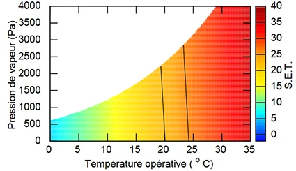
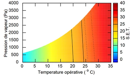
$$ C + R + E = \frac{1}{R_{\text{g}} + R_\text{cl}} \times (T_\text{sk} - SET^* ) + \frac{\omega }{R_{\text{e}}}\times \Big (p_\text{sk} - 50 \\% p_\text{vs}(SET^*) \Big) $$Figure 8 shows SET as a function of humidity and temperature. It can be seen that comfort is dependent on humidity: at the same operating temperature, the SET is greater at high humidity than at low humidity. The range of comfortable SET was determined by comparing the model with an experimental campaign and goes from 22.2 to 25.6°C [Nishi, 1977]5.
Effect of environment on comfort
Semi-open spaces are subject to wide variations in ambient conditions, including air velocity and average radiant temperature. This section therefore focuses on their effects on simulated physiological reactions.
Air velocity and clothing properties
Thermal resistance and vapour permeation resistance are actually affected by the “pumping” effects associated with the wearer’s movement, which promote air intake into clothing, and by wind-related air movements. This reduces their convective properties and their resistance to water vapour transfer. The following paragraphs describe the calculation of the decrease in these resistances according to ISO 9920, the genesis of which is described in [Holmer, 1999] and [Havenith, 1999] .
Variation in thermal resistance
The decrease in resistance to heat transfer is defined in [Holmer, 1999] . For a walking velocity smaller than \(v_{\text{w}} < 0.7\) [m/s] (i.e. 2.5 [km/h]) an equivalent walking speed is defined \(v_{\text{w}}\) depending on the activity level \(M\):
$$ v_{\text{w}} = 0.0052 \times (M - 58) $$For the convective heat transfer coefficient \(h_{\text{c}}\) the corrected velocity \(v_{\text{c}}\) should be used, taking into account the air velocity \(v\) and the walking velocity \(v_{\text{w}}\):
$$ v_{\text{c}} = \sqrt{ v^2 + v_{\text{w}} ^2} $$The corrected total convective thermal insulation and insulation of clothing \(R_{\text{T}}= R_{\text{g}} + R_\text{cl}\), which is valid between 0.2 and 3 [m/s] and \(clo \ge 0.6\) is provided from following correlation:
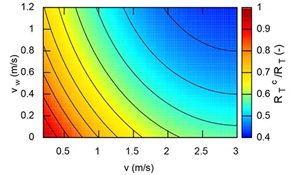
$$ \frac{R_{\text{T}}^{c}}{R_{\text{T}}} = \exp \left( 0.043 - 0.398 \times v_{\text{c}} + 0.066\times v_{\text{c}}^2 - 0.378 \times v_{\text{w}} + 0.094 \times v_{\text{w}}^2 \right) $$Where \(R_{\text{T}}\) is the thermal insulation of clothing and the ambient air layer, with the thermal resistance value of clothing at zero air velocity \(R_\text{cl}\). The convective thermal resistance is calculated with \(v \sim 0\) [m/s]
An illustration of the ratio \(R_{\text{T}}^{c}/R_{\text{T}}\) is shown in Fig. 9 as a function of air and walking velocities. It can be seen that an air velocity of \(\sim 1\) [m/s] at zero walking speed results in a significant reduction of \(\sim 25 %\) resistance to thermal transfer. It is therefore important to recalculate the heat transfer taking this reduction into account in order to obtain an accurate heat balance.
Variation of the vapour permeation resistance
Corrected vapour transfer permeability \(i_{\text{m}}^c\) is given by [Havenith, 1999] :
$$ \frac{i_{\text{m}}^{c}}{i_{\text{m}}} = 4.9 - 6.5 \Big( \frac{R_{\text{T}}^{c}}{R_{\text{T}}} \Big) + 2.6 \Big ( \frac{R_{\text{T}}^{c}}{R_{\text{T}}} \Big)^2 $$The variation in the permeability index \(i_{\text{m}}\) depending on \(\frac{R_{\text{T}}^{c}}{R_{\text{T}}}\) is shown in Fig. 10. This illustration shows that for a 70% reduction in heat transfer, vapour permeability \(i_{\text{m}}^c\) is multiplied by \(\sim 1.6\) compared to \(i_{\text{m}}\) in a quiet atmosphere. The equation giving the resistance to steam transfer \(R_{\text{e}}\) is modified and has a significant impact on the latent energy balance.
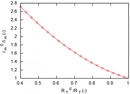
Fig. 11 shows the difference between SET calculated with constant (solid line) and variable (dotted line) clothing properties calculated from the previous equations, for an air velocity of \(v= 1\) [m/s]. A shift from the comfort zone to higher temperatures occurs: clothing properties are reduced, sensitive and latent transfers are increased and the operating temperature must be higher in order to obtain the same flow lost on the skin surface.
Influence of the average radiant temperature
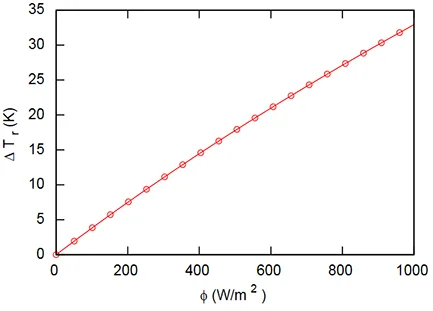
The last equation of Radiative Exchanges section gives the average radiant temperature increment \(\Delta T_{\text{r}}\) depending on the solar fluxThe vapour flow rate incident on the person. Thus, for 600 [W/m²] of incident flux, we observe an increment of \(\sim 26\) [K] with respect to the radiant temperature without sunlight.
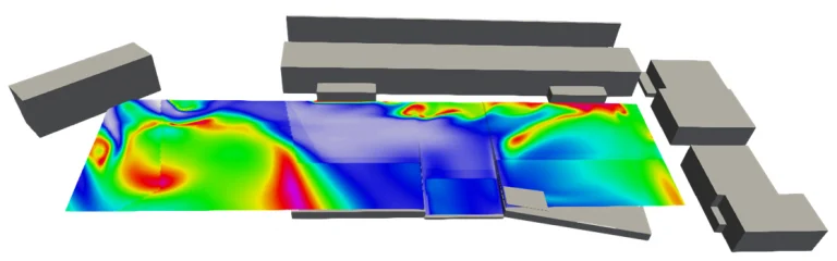
An illustration of the influence of the average radiant temperature and air velocity is given in Fig. 13, where the SET comfort indicator is given spatially. The radiant temperature is calculated from the ground temperatures and the incident solar flux. For this example, air velocities were calculated by the mechanics of the computational fluids. It has been assumed that air temperature and humidity are not affected by the urban environment. The disparity of SET shows the important effect of air velocities and average radiant temperatures.
Influence of physiological variability on SET
As we have seen in the previous sections, SET is calculated from an individual’s physiological reactions. In the standard [ASHRAE, 2013] , these reactions are those of a male individual. As the morphological parameters are adjustable, it is possible to use the model for other phenotypes and to evaluate the comfort resulting from their physiological reactions.
The model presented for the control of the metabolism has a large number of parameters. In order to show the sensitivity of the model to them, the effects of the variability of physiological parameters on the SET comfort indicator evaluated from random draws are presented here. The dispersion of the results will be assessed in terms of standard deviation: it should be kept in mind that \(\pm 2\) standard deviations around an average value correspond to 95% of the population assessed.
Presentations of variable physiological parameters
Many physiological characteristics can be accurately represented by Gaussian statistical distributions (e.g. size, mass). Assuming that this is also the case for other model parameters, the Monte Carlo method was used to assess the dispersion of SET resulting from physiological variability.
The variable parameters chosen for the variability assessment are as follows:
- size, mass and percentage of fat mass,
- the coefficients \(C_\text{d}\), \(C_\text{s}\), \(C_\text{sw}\), \(C_\text{sh}\) respectively for dilation, tightening, sweating and tremor,
- the conductance of fabrics \(U_\text{sk}\) and basal blood flow \(q_\text{b}^\text{set}\),
- the setpoint core and skin temperatures \(T_\text{c}^\text{set}\), \(T_\text{sk}^\text{set}\).
The dispersion around mass and size was chosen from data from INSEE. The average value of the other parameters is that of the original code. For the target skin and core temperatures, the standard deviation is considered to be 0.5% of the mean value in order to respect the minimum and maximum internal temperature values recorded by [Mackowiak, 1992]16.
For the other parameters, the standard deviation is taken to be 5% of the mean value, which is a conservative assumption given the disparities observed for the dilation constant, for example. Tissue conductance can also vary to a greater extent [Schweiker, 2017]17. The table below summarises the numerical values used.
Parameters considered as variable in the Pierce’s model:
| Parameter | Mean value $\mu$ | Standard deviation $\sigma$ |
|---|---|---|
| Height [m] | 1.75 | 0.065 |
| Mass [kg] | 71.4 | 8.9 |
| Fat [%] | 23 | 7.5 |
| \(C_{\text{d}}\) [L/m².h.k] | 200 | 10 |
| \(C_{\text{s}}\) [1/K] | 0.5 | 0.025 |
| \(C_{\text{sw}}\) [kg/(m².h.K)] | 170 | 8.5 |
| \(C_{\text{sh}}\) [kg/(m².K)] | 19.4 | 0.97 |
| \(U_{\text{sk}}\) [W/(m².K)] | 5.28 | 0.264 |
| \(q_b^{\text{set}}\) [L/(m².h)] | 6.3 | 0.315 |
| \(T_{\text{sk}}^{\text{set}}\) [°C] | 33.7 | 0.169 |
| \(T_{\text{c}}^{\text{set}}\) [°C] | 36.8 | 0.184 |
The resulting SET differences are presented in the following sections.
Gender effect
The difference in comfort temperature between women and men has been studied experimentally and numerically [Kingma, 2015]18 [Hoof, 2008]19. Here, the average SET for male and female individuals is calculated from random draws on parameters according to Gaussian laws described later . Basal metabolism is calculated according to the very first equation based on the size and mass of each individual and the level of clothing chosen is 1 [clo].
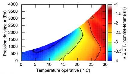
The average SET difference between the two genders is shown in Fig. 14 for operating conditions, i.e. \(T_{\text{a}} = T_{\text{r}}\) at a low air velocity of \(v=0.1\) [m/s]. The difference between average SET ranges from -4 to -1.25 [K] for the studied conditions.
In the range between 19 and 25°C of operating temperature which contains the comfort zone defined according to[Nishi, 1977]5 - see Fig. 8 - the average gender difference varies from -3.5 to -2 [K]. The average SET calculated for men and women therefore differ significantly and in some cases this difference is larger than the comfort zone, which is 3.4 [K].
It should also be noted that according to the results of the model, the SET obtained for women is higher than that of men: this implies that a higher operating temperature of the reference environment is required to produce the same physiological reaction as in men.
Environment effect
In this section, the effect of the variability of a population with both sexes equiprobably distributed is presented. Physiological parameters are distributed according to Gaussian distributions as described in 5.1. The clothing is 1 [clo] and the activity is 1 [met].
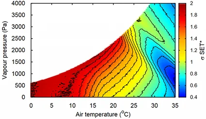
The standard deviation of the SET distributions obtained at any point in the psychrometric diagram is plotted for high wind conditions (\(v=1\) [m/s]) on Fig. 15. It can be observed that the standard deviation can vary from \(\sim\) 0.4 à 2 [K]. This implies that under these conditions, the temperature felt by 95% of the population varies between 1.6 and 8 [K], or four standard deviations.
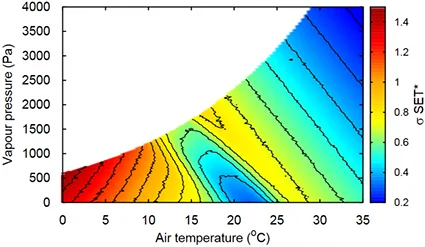
The standard deviation obtained for high solar flux conditions, i.e. \(T_{\text{r}}=T_{\text{a}} + 30\) and a low air velocity \(v=0.1\) [m/s] are shown in Fig. 16. We observe that it varies between \(\sim 0.2\) and \(1.4\) [K], which implies that 95% of the population is in a range between 0.8 and 5.6 [K] under conditions of high radiant temperature.
While these ranges may seem extensive, the literature review of [Hoof, 2008]19 mentions experimental campaigns where deviations of \(10\sim\) [K] were recorded between temperatures declared comfortable. In indoor environments, it is therefore difficult to define a setpoint temperature adapted to each individual. In outdoor space, it is appropriate to integrate variability into the estimation of comfort, in the spirit of [Bruse, 2007]20.
Conclusion
This article exposes the fact that the determination of comfort in environments with variable conditions requires an appropriate indicator, allowing the calculation of metabolic reactions in transient conditions.
Clothing also plays a significant role in the heat and moisture balance of the human body. Its transfer properties being highly variable with wind speed, it is necessary to obtain an appropriate estimate of air velocity around the body in (semi-) outdoor spaces.
Morphological characteristics such as gender, mass, height also have a significant influence on the numerical evaluation of comfort by the SET model. A significant variation in perceived comfort can be introduced by physiological variability, especially in outdoor conditions where high air velocities and strong solar radiation are often encountered.
In this article, a dynamic model of the human body for the calculation of comfort has been presented. Other models exist and can be used, including the Physiological Equivalent Temperature (PET). The latter uses many of the equations of the two-nodes model presented here, as well as a similar reference environment. However, PET is defined as the temperature of an environment that would produce the same skin and core temperatures as the environment being studied.
Other more complex models have been developed, ranging up to 340 nodes [Fiala, 1999]21 leading to the comfort index named Universal Thermal Comfort Index (UTCI). However, the complexity of the model does not make it of the practical nor provides an easy calibration of physiological information, particularly if variability is to be incorporated. A correlation based on multiple linear regressions has nevertheless been derived and allows us to evaluate the comfort of a pedestrian walking at a speed of 4[km/h].
The individual’s thermal history also has an influence on his or her feelings: for example, one appreciates an atmosphere at 16°C for a few minutes after making an intense effort, while the same atmosphere would be considered too cold when the body is in thermal balance. The approach to alliesthesia developed by [Parkinson, 2012]22 proposes a model for this phenomenon. The notion of “pleasure” felt during alliesthesic phenomena also goes beyond the usual approach, which focuses on thermal neutrality.
The psychological aspects of comfort should also not be neglected: it has been proven that under identical conditions, the feeling of comfort is better in a furnished room (furniture, decoration) than in a bare room [Rohles, 2007]23. Similarly, the placebo effect has an impact: when the user thinks he or she has control over the set temperature, his or her feeling is positively affected, whether or not this control is effective [Rohles, 2007]23.
In this sector, local comfort features such as heaters, heated seats, office fans or seat-mounted fans provide an interesting response to the variability in comfort temperatures. Considerable energy avings have been achieved at a pilot site [Brager, 2015]24: by providing each individual with a power of around 20 Watts, the decrease in the overall setpoint temperature has resulted in a power reduction of 500 W/person.
The source code of the SET and PET comfort indexes can be dowloaded in the Tools dropdown menu ! Et voilà 😉
Vernon, H. M. (1936), Accidents and their Prevention, DOI ↩︎
Fanger, P. O. (1970), Thermal Comfort: Analysis and applications in environmental engineering, Copenhagen: Danish Technical Press ↩︎ ↩︎
Van Hoof, J. (2008), Forty years of Fanger’s model of thermal comfort: comfort for all?., Indoor air, 18(3), 182-201. ↩︎
Gagge, A. P. (1936). The linearity criterion as applied to partitional calorimetry. American Journal of Physiology-Legacy Content, 116(3), 656-668. ↩︎
Nishi, Y., & Gagge, A. P. (1977). Effective temperature scale useful for hypo-and hyperbaric environments. Aviation, space, and environmental medicine, 48(2), 97-107. ↩︎ ↩︎ ↩︎
Höppe, P. (2002). Different aspects of assessing indoor and outdoor thermal comfort. Energy and buildings, 34(6), 661-665. DOI ↩︎
Part, V. (2008). I: Environmental meteorology, methods for the human-biometeorological evaluation of climate and air quality for the urban and regional planning at regional level. Part I: Climate. Part I: Climate. VDI/DIN-Handbuch Reinhaltung der Luft, 29. DOI ↩︎
Schiavon, S., & Lee, K. H. (2013). Dynamic predictive clothing insulation models based on outdoor air and indoor operative temperatures. Building and Environment, 59, 250-260. DOI ↩︎
A.P. Gagge, J.A.J. Stolwijk, Y. Nishi, Effective temperature scale based on a simple model of human physiological regulatory response, ASHRAE Trans. 77 (1971) 247– 263. ↩︎
Cain, J. B., Livingstone, S. D., Nolan, R. W., & Keefe, A. A. (1990). Respiratory heat loss during work at various ambient temperatures. Respiration physiology, 79(2), 145-150. DOI ↩︎
Helbig, A., Baumüller, J., & Kerschgens, M. J. (Eds.). (2013). Stadtklima und Luftreinhaltung. Springer-Verlag. ↩︎
Fobelets, A., 1988, Rationalization of the Effective Temperature \(ET^\) as a Measure of the Enthalpy of the Human Indoor Environment*, ASHRAE Transactions ↩︎
ASHRAE, 2009, ASHRAE Handbook, Fundamentals. Chapter 6: Mass transfer ↩︎
Höppe, P. R., 1993, Heat balance modelling. Experientia, 49, 741-746. ↩︎
ASHRAE, 2009, ASHRAE Handbook, Fundamentals. Chapter 9: Thermal Comfort ↩︎
Mackowiak, P. A., Wasserman, S. S., & Levine, M. M., 1992. A critical appraisal of 98.6 F, the upper limit of the normal body temperature, and other legacies of Carl Reinhold August Wunderlich. Jama, 268(12), 1578-1580. PDF link ↩︎
Schweiker, M., Fuchs, X., Becker, S., Shukuya, M., Dovjak, M., Hawighorst, M., & Kolarik, J. (2017). Challenging the assumptions for thermal sensation scales. Building Research & Information, 45(5), 572-589. PDF link ↩︎
Kingma, B., & van Marken Lichtenbelt, W. (2015). Energy consumption in buildings and female thermal demand. Nature climate change, 5(12), 1054-1056. PDF Link ↩︎
Van Hoof, J. (2008). Forty years of Fanger’s model of thermal comfort: comfort for all? Indoor air, 18(3), 182-201. PDF Link ↩︎ ↩︎
Bruse, M. (2007, November). Simulating human thermal comfort and resulting usage patterns of urban open spaces with a multi-agent system. In Proceedings of the 24th International Conference on Passive and Low Energy Architecture PLEA (Vol. 24, pp. 699-706). PDF Link ↩︎
Fiala, D., Lomas, K. J., & Stohrer, M. (1999). A computer model of human thermoregulation for a wide range of environmental conditions: the passive system. Journal of applied physiology, 87(5), 1957-1972. PDF Link ↩︎
Parkinson, T., De Dear, R., & Candido, C. (2012, April). Perception of Transient Thermal Environments: pleasure and alliesthesia. In Proceedings of 7th Windsor Conference, Windsor, UK (No. 56). PDF Link ↩︎
Rohles, F. (2007). Temperature & Temperament. American Society of Heating, Refrigerating and Air-Conditioning Engineers, 14-19. PDF Link ↩︎ ↩︎
Brager, G., Zhang, H., & Arens, E. (2015). Evolving opportunities for providing thermal comfort. Building Research & Information, 43(3), 274-287. PDF Link ↩︎