Climate data and meteorology
This page aims to clarify some points about historical meteorological data sources, their origins, as well as prospective meteorological / climate data.
In engineering studies, particularly in HVAC (Heating, Ventilation, Air Conditioning) and thermal studies (regulatory or not), meteorological files that are representative of the current climate are used to accurately size technical installations, such as heating systems. These are files with hourly time steps for a complete year. These files are referred to as TMY (Typical Meteorological Year).
Today, it is sometimes requested to simulate a specific year, e.g. the heatwave of 2003, to verify the resilience of a building or to check the associated comfort levels. However, this type of file is not used in classic technical sizing.
To obtain this type of files, historically, meteorological measurement stations were used, either by taking a specific year (AMY files) or by taking statistics over several decades (TMY files).
However, for questions of spatial precision (there is not a meteorological station at every corner!), to make short-term weather forecasts (typically for weather bulletins) or long-term forecasts (climate evolution), climate models have been developed over the past fifty years. These models allow for a better understanding of global phenomena, prospective analysis (for example, with the famous IPCC scenarios), and to enrich the data measured at meteorological stations.
These different approaches complement each other, as shown below.
Meteorological measurements
A meteorological station refers to a set of sensors that record and provide physical measurements and meteorological parameters related to climate variations for a specific location.
The variables usually measured are temperature, pressure, wind speed and direction, humidity, dew point, rainfall, cloud height and type, type and intensity of precipitation, and visibility. Stations may include sensors for all or only some of these parameters, depending on their type: agro-meteorological, airport, road weather, climatological, etc.
The measurement of solar radiation is occasional and is not part of the essential measurements defined by the World Meteorological Organization (WMO) although they are indispensable as input data for thermal simulations. These data can come from independent observation networks or data reconstructions.
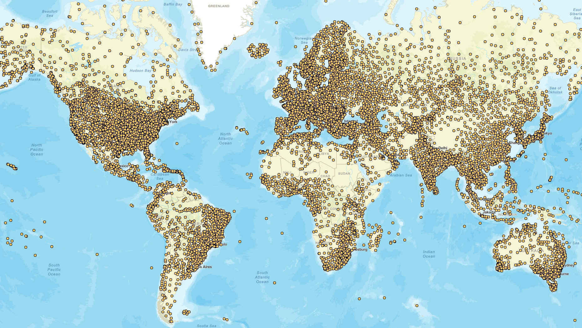
Source: NCEI/NOAA
There are several measurement networks, including national networks that share all or part of their data with the WMO (such as Météo France) or professional networks like the ICAO (International Civil Aviation Organization).
Stations generally have a WMO identifier, and/or sometimes an ICAO identifier.
These data are increasingly accessible today, for example through the following links (non-exhaustive list)
- meteostat : access to historical, hourly, or daily data for the entire world.
- Météo France : access to various types of data and indicators from measurements and/or models.
- NOAA (National Oceanic and Atmospheric Administration - USA) : centralization of global data measured by WMO members. It notably includes hourly data.
Weather models
In theory, the planetary climate could be simulated as a whole by incorporating all time and space scales. However, this would be numerically too heavy; to date, there are no computers with enough computing capacity to process such large amounts of data.
Therefore, we proceed with scale separations, creating cutoffs at characteristic sizes that have physical meaning in terms of what can be measured and validated.
Starting from the coarse to refined, there are three scales: global, regional, local.
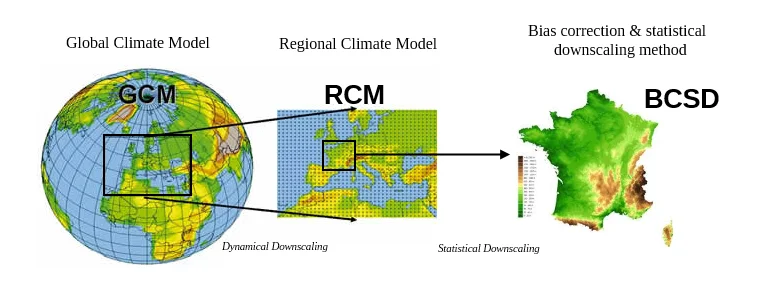
Source: DRIAS
Global Models, GCM (General Circulation Model)
The entire globe is simulated, with coarse grids, with approximately 80 km in height. Different variants of these models exist, depending on the intended use.
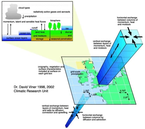
Source: IPCC
- GCM Global Circulation Model: This is a global model with coarse grids, used to provide long-term trends over large areas.
- AGCM Atmospheric Global Circulation Model: This is a specific category of GCM that only takes the atmosphere into account. This provides valid predictions only as long as other components (soil, oceans, ice) remain unchanged. In practice, these are the models used for weather forecasting.
- AOGCM Atmospheric Oceanic Global Circulation Model: This is another category of GCM that takes both the atmosphere and the ocean into account. It is sometimes also referred to as Atmospheric Oceanic Global Coupled Model, because these models not only consider the ocean but also the interactions between the ocean and the atmosphere. These are the models used in climatology.
There are currently about fifteen global models around the world: HadCM3, EdGCM, GFDL CM2.X, ARPEGE-Climat, etc.
The data from this family of models can then serve as input data for the following models, by forcing boundary conditions at a lower scale.
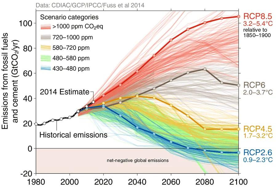
This type of model is used for prospective climate studies, for example by modifying CO2 levels in the atmosphere and analyzing the impact this can have on other meteorological variables: typically the IPCC scenarios!
Regional Models, RCM (Regional Climate Model)
The main advantage of regional climate models is to limit the computational cost of simulations compared to global climate models of the same resolution. They allow for a finer exploration of climate representation and climate change. There are many models of this type, including: Aladin (MF), ARPEGE (MF), RACMO22, HAadGEM2, IPSL-CM5, MPI-ESM, NorEMS1, etc.
They also allow precise time series generation.
Classical weather forecasts are derived from this type of approach.
Local Downscaling
Two main families of methods allow for downscaling to a very local level: either through simulations (dynamic) or statistically.
Bias Correction and Dynamic Downscaling
In order to account for more precise physical phenomena and consider more interactions, dynamic approaches use the results of RCM scales as input data (boundary conditions) to simulate finer scales.
Different simulation models exist to perform this downscaling.
At L’hypercube, the WRF model has been chosen.
- Main advantages of these approaches:
- They represent more physical phenomena,
- Few assumptions,
- They ensure consistency between meteorological variables.
- Disadvantages:
- They are computationally heavy,
- The results depend heavily on the quality of the input data.
Bias Correction and Statistical Downscaling
The other family of approaches is statistical downscaling.
These approaches have developed significantly because they are computationally inexpensive.
Main advantages of these approaches:
- Very computationally efficient,
- Can take into account a lot of input data from GCMs / RCMs,
- The results produced are consistent with meteorological observations.
Disadvantages:
- They are not the most suitable for studying climate change,
- Possible introduction of numerical artifacts.
In France, the ADAMONT model is quite commonly used.
Assimilation Models: The Best of Both Worlds
These are approaches that assimilate real (measured) data into GCM or RCM simulations, allowing for the determination of temperature (and other meteorological quantities) in each grid cell of the globe (grid cell of about 30km). This way, it is possible to obtain time series for any point on the globe, which are consistent with each other.
Among the existing models, we find: ERA5 (Europe) the most recent, ERIA, MERRA (NASA), CFSR, etc.
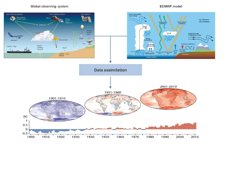
Source: ECMWF
Hourly Meteorological Files for a Typical or Real Year
In practice, how do we go from measurement networks and models at more or less large scales to meteorological files usable by thermal / comfort / etc. softwares?
Files Representing the Current Climate: TMY (Typical Meteorological Year)
These are the standard files for regulatory studies. They are representative of the current climate (generally an average over the last 20 to 30 years) and are presented in the form of a typical year with hourly values.
These are reconstructed files, with real months from different years that are statistically equivalent to the average of the last 20 years.
TMYx: created by Climate.OneBuilding.org , a reference site. These are data derived from real surface temperature measurements according to the TMY/ISO 15927-4 methodology. Based on measurements, observations, and reanalyses of solar radiation from ERA5 (an atmospheric model adjusted with observations).
The TMYs used at AREP are mainly derived from the software Meteonorm :
- Solar radiation is based on averages over the period 1996-2015.
- Other quantities are based on the period 2000-2019.
These are the files used in regulatory studies (RT2012 / RE2020 calculations in France).
Available Quantities:
| Variable | Unit | Informations |
|---|---|---|
| Dry Bulb Temerature | °C | - |
| Dew Point Temperature | °C | - |
| Relative Humidity | % | - |
| Atmospheric Station Pressure | Pa | - |
| Extraterrestrial Horizontal Radiation | Wh/m² | - |
| Extraterrestrial Direct Normal Radiation | Wh/m² | - |
| Horizontal Infrared Radiation from Sky | Wh/m² | - |
| Global Horizontal Radiation | Wh/m² | - |
| Direct Normal Radiation | Wh/m² | - |
| Diffuse Horizontal Radiation | Wh/m² | - |
| Global Horizontal Illuminance | Lux | - |
| Direct Normal Illuminance | Lux | - |
| Diffuse Horizontal Illuminance | Lux | - |
| Zenith Illuminance | Cd/m² | - |
| Wind Direction | °/North | North: 0°, East: 90°, … |
| Wind Speed | m/s | - |
| Total Sky Cover | - | 1 is 1/10 covered. 10 is total coverage |
| Opaque Sky Cover | - | 1 is 1/10 covered. 10 is total coverage |
| Visibility | km | - |
| Ceiling Height | m | - |
| Precipitable Water | mm | - |
| Aerosol Optical Depth | - | in 1/1000 |
| Snow Depth | cm | - |
| Days Since Last Snowfall | days | - |
| Albedo | - | |
| Precipitation Depth | mm | - |
| Precipitation Quantity | hr | - |
Year N Files
As mentioned at the beginning of this page, there are now many open databases of real data.
Within L’hypercube, these data are widely used when studying wind in urban environments, where statistics must be based on real measured data, but also widely for the precise evolution of temperatures and humidity studies.
Most of the quantities described previously can be found here, but some quantities like solar radiation are not always measured. Thus, it is sometimes necessary to reconstruct files by mixing measurements from one year with radiation from a typical year, or simulated radiation from atmospheric models.
It is not always possible to find complete meteorological files for a year N for free.
This type of file is sometimes used in advanced STD studies, especially when there are questions about comfort and adaptation to climate change.
It is common, for example, to resimulate a building with the 2003 heatwave to verify its resilience to climate change.
Future Climates - IPCC Scenario
To obtain future climates in the form of meteorological files, the logic is to assume the evolution of one or more parameters on a very large scale, and through simulation and downscaling, see the local impact.
Among the most well-known are the IPCC CO2 emission scenarios, which have been integrated into GCMs. These forecasts have then been localized through downscaling (RCM and possibly a step of dynamic or statistical downscaling). Thus, depending on the emission scenarios considered (RCP2.6, RCP4.5, or RCP8.5), one can look ahead at future meteorological data.
This need to extract data from GCM or RCM is the reason why there are no simple approaches today to perform morphing of weather files (a kind of tool that would take a current weather file as input to transform it into a future weather file).
Within AREP, the Meteonorm tool is used to obtain these files.
For these prospective scenarios, the same distinction of files is found:
- Future TMY files, representative of the average climate at a given horizon,
- Future “real year” files.
TMY-2XXX Files
Similar to TMY files representative of the current climate, we first find future TMY files. That is, for weather representative of the climate in 2080, for example, we actually consider the average climate between 2070 and 2090.
The information contained in these types of files is very useful, especially for verifying the overall behavior of buildings and projects with respect to global climate changes. However, due to the averaging over approximately two decades, extreme events generally do not appear in them.
Within AREP, these files are used for prospective comfort studies.
Year 2XXX File
Due to the methodology employed during the development of prospective scenarios and the use of GCMs (followed by downscaling), in reality all future years are simulated, making it possible to retrieve specific years.
This makes two approaches possible when looking for specific climatic years. Keeping the previous example of 2080, using different GCMs, with different assumptions (e.g., RCP 4.5 and RCP8.5) and possibly different downscalings to generate a sort of database of weather files around 2080:
- Either by keeping all the years and all the model variations, and selecting the worst,
- Or by keeping the year that is at the 90th or 95th percentile of the entire database.
Within AREP, this type of approach is beginning to be used for thermal comfort and adaptation studies.
Adaptation to Climate Change
What about DRIAS data then (France specific)?
The DRIAS project (Providing access to French Regionalized climate scenarios for the Impact and Adaptation of our Societies and environment) provides indicators of warming and more generally of climate changes for different horizons, at large scales. They use the methods described above: GCMs, RCMs, and data assimilation.
The presented information is the regionalized data of the most recent climate projections produced by climate research actors in France (CERFACS, CNRM, IPSL), particularly the SCAMPEI project. The parameters and indicators (number of abnormally hot nights, number of frost or heatwave days, etc.) are represented at a resolution of 8 km across metropolitan France.
Discovery section: access to mapped indicators, including indicators related to TRACC (see below)
Example of analysis available on the DRIAS website. Data and Products section: access to temporal files (
csvornetcdfformats), which map the entire metropolitan territory, down to grids of a few kilometers.
And what about TRACC ?
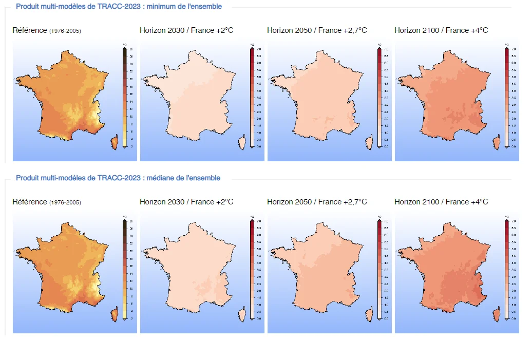
TRACC: Reference Warming Trajectory for Climate Change Adaptation
The TRACC represents a paradigm shift: we no longer look at climate evolution up to a certain date, but we consider warming scenarios.
In the main scenario adopted, global warming continues and stabilizes at +3°C by 2100 compared to the pre-industrial era, which is about +4°C on average over metropolitan France. This scenario corresponds to the continuation of existing global policies, without additional measures.
The TRACC scenario in France roughly corresponds to an RCP8.5 scenario by 2100. These data and scenarios are available on the DRIAS website.