Urban Heat Island

icu strasbourg — *Fig. 1: Illustration of comfort levels in a dense urban environment: Strasbourg station forecourt*

Phenomenon

The city is subject to the urban heat island (UHI) phenomenon, which is characterized by higher temperatures in the conurbation than in the countryside. This difference is due to both the geometric characteristics and the type of surfaces, different in each environment:

Radiation trapping occurs during the day, when reflections of the sun’s rays on built surfaces increase the amount of energy absorbed, as well as at night, due to the relative narrowness of the streets in relation to the façades, inhibiting radiant cooling towards the sky vault.
The tortuosity of the streets limits the wind speed compared to an open environment and thus reduces the cooling of the surfaces by convection.
The high proportion of mineral surfaces in the urban environment implies it stores more heat than vegetation, making night-time cooling less effective.
Evapotranspiration originating from low or high vegetation (i.e. the fact that it liberates water as vapour

hence the need for watering) helps to keep foliage temperatures relatively low. The shade provided by tree crowns also results in lower temperatures compared to a soil without a vegetated canopy.

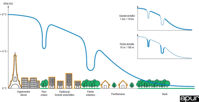
The UHI phenomenon is illustrated in the following figure, taken from the “Cahiers de l’ APUR ” and representing the temperature difference between the centre of Paris and the surrounding rural environment.

APUR ICU — *Fig. 2: Illustration of the UHI, taken from APUR*

In the context of global warming, which leads to an increase in the frequency and intensity of heatwaves, it seems imperative to be able to anticipate the temperature and comfort levels in the city of tomorrow.

In brief, different types of numerical models exist to predict the urban climate, from the regional to the street scale:

The TEB model developed at CNRM makes it possible to simulate air temperature changes on a large scale by coupling an urban canopy model with simplified “canyon” streets comprising a unidirectional heat transfer model from the ground to the canopy.
Coupled simulation tools, such as SOLENE-micro climat or ENVI-MET allow a higher level of detail for modelling the urban environment and offer a coupled resolution of convective and radiative heat transfer with anisothermal air simulation. This approach, which includes the dynamic thermal behaviour of buildings and their equipment as well as water-content balances on vegetation, has the distinct advantage of accuracy. The computational cost is nevertheless high, with calculation times of the order of several tens of hours for a simulated time of the order of a week

The experience of the design process shows that it iterative is by nature: thus many project variants need to be evaluated. It is therefore necessary to have both a sufficiently detailed model for the assessment of the impact variants on the thermal behaviour of a space, and a fast enough tool allowing for the sensitivity analysis of parameters required during the design process.

A “simple” way: weak coupling

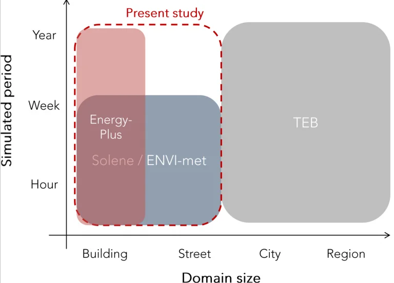
In order to meet this need to iterate, an alternative model was developed within the team, based on a decoupling of the thermal and aeraulic calculations. The idea is to make an additional use of the air velocity field originating from the CFD computations and to improve the accuracy of the calculation at a lower cost. The open softwares EnergyPlus and openFOAM are used to this end. The method developed aims at allowing an annual simulation of the phenomenon, in articular to evaluate the frequency of heatwaves over a full summer season. In terms of spatial scale, the simulation is carried out from the building to the neighbourhood. The following figure illustrates this situation as well as the time and space scales addressed by the existing tools.

Thermal model

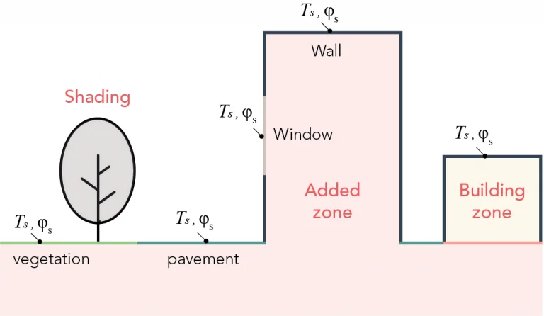
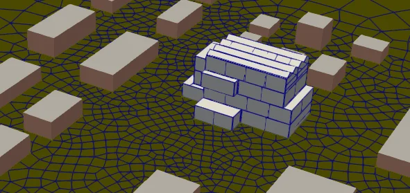
The capabilities of the EnergyPlus building simulation engine are used to obtain the incident solar fluxes at the façade and the temperatures of the different surfaces according to their composition (albedo, material, thickness, glazing…). Thus, the buildings are represented by distinct “thermal zones”, the low vegetation is simulated with a “green roof” model incorporating the complete water balance and the trees are assumed to be mere shading obstructions (we assume they do not emit water vapour). The following figure illustrates the principle of the model.

Zones themriques — *Fig. 4: Sketch of the different thermal zones or objects in the approach developed.*

The integration of view factors in the radiation model was also developed using the SurfaceProperty:SurroundingSurfaces object in the EnergyPlus model, in order to improve the prediction. And since the publication of our opensource pyViewFactor Python library, their exact computation is possible and they can be introduced into the EnergyPlus framework.

Air flow

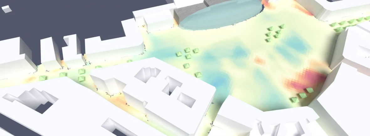
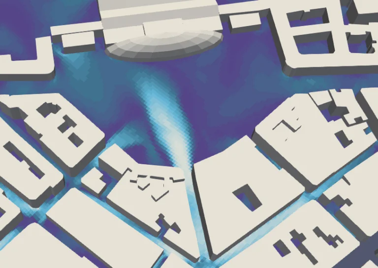
The “numerical wind tunnel” approach described in detail here is implemented in order to calculate the velocity fields at an hourly scale, in compliance with the guidelines for such modelling practices. An example of results is provided below, showing the amplitude of the air velocity at a given time on the forecourt of Strasbourg station.

Strasbourg aero — *Fig. 5: Wind velocity field at a given time on Strasbourg's station forecourt.*

A by-product : local convection coefficients

An interesting by-product of the airflow simulation is the local air velocity near the walls, which can be fed back to the building simulation model.

The animation below show the surface temperature differences with/without local convection coefficients during the first week of the year. One can see the noticeable effect of wind-driven convection, with +/- 4[K] of variation of surface temperatures.

Coefficients locaux — *Fig. 6: Temperature differences with/without local heat exchange coefficients for a test case.*

Yet another by-product: urban surroundings influence on energy consumption

Simulating the urban scene as a whole with a separation of thermal zones gives the energy consumption per building (heating, cooling, electricity) in addition to the outdoor comfort level, allowing for a holistic approach of the problem.

scene urbaine — *Fig. 7: 3D model of buildings within an urban scene.*

Weak coupling principle

In order to avoid long, costly, anisothermal CFD calculations, we propose to neglect the influence of buoyancy on air movements: we assume that the air speed prevails over the temperature difference between the air and the surfaces in contact with it. In other words, natural convection is neglected.

This strong assumption is true in the presence of wind and wrong in its absence. However, this modelling approach, while not exact, considerably reduces the computational effort and, to us, appears more relevant than not doing the calculation at all.

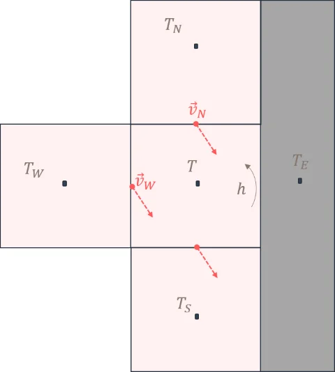
Under this assumption, the problem reduces to a “simple” steady state heat balance for each cell of the mesh (see figure below for the 2D case), in accordance with the principle of conservation of energy.

This simplified approach allows for the resolution of both scalar temperature and humidity fields. hus the influence of evapotranspiration on temperature and the amount of water vapour in the ambient air are taken into account.

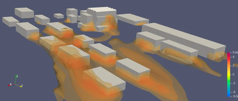
An example of the result is shown in the figure below, showing isovolumes being 2°C higher than the air inlet temperature in the meshed volume. The increase in air temperatures can be seen in the recirculation zones behind the buildings (i.e. downstream in the present case).

couplage — *Fig. 9: Temperature deviation from the inlet temperature in the fluid domain: influence of recirculation zones.*

A word on solar flux absorption by water

In the following sections, details are provided on the modelling of solar radiation absorbed by water. Indeed, the phenomenon is seldom dealt with in the educational literature, hence we thought it would be of some use to expose it here.

Problematization

The solar radiation consists of wavelengths of the order of 0.1 < $\lambda$ < 2.5. These are absorbed differently by the media they pass through, like infrared rays which are absorbed and reflected by glass (opaque to infrared radiation), thus producing the greenhouse effect.

Solar flux is considered as totally absorbed after $\sim$ 90 [m] in water. The fraction of remaining energy at this depth is however very small: after $\sim$ 2 [cm], 25% of radiation is already absorbed, mainly in the infrared domain [ Rabl & Nielsen 1975 ].

The following points can be made:

infrared radiation is integrally absorbed within the first centimeters,
short wave radiation penetrates up to, $\sim$ 90 [m],
at a depth of 10 [cm], 45% of radiation is absorbed,
at a depth of 1 [m], 65% of radiation is absorbed.

It is therefore necessary to have a model that can represent absorption as a function of depth, differentiated according to the wavelength band considered.

Radiative absorption model

Solar flux is absorbed differently depending on the wavelength of the spectrum. [ Kaushik 1980 ] proposes a formulation where the transmissivity as a function of depth is presented as the sum of the transmissivities in five different wavelength bands, such that

$$ \tau (z) = \sum_{i=1}^{5}\mu_i\exp^{-\nu_i z} $$

The coefficients $\mu_i$, $\nu_i$ for each wavelength band are given in the following table.

Wavelength band [µm]	Fraction of solar enrgy $\mu_i$ [-]	Extinction coefficient $\nu_i$ [1/m]
0.2-0.6	0.237	0.032
0.6-0.75	0.193	0.450
0.75-0.9	0.167	3
0.9-1.2	0.179	35
1.2-50	0.224	255

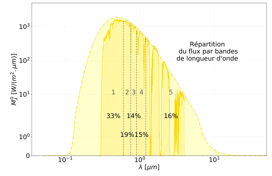
One can see that the fraction of the solar spectrum per wavelength band represented by coefficient $\mu_i$ is close to the fraction of energy comprised in the reference solar spectrum ASTM G-173 as indicated on following figure (on the latter, the theoretical black body spectrum of the sun is also drawn).

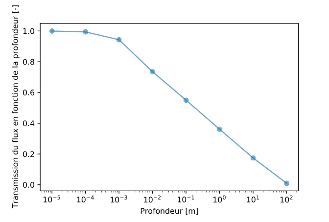
M0k2 — *Fig. 10: Energy of the ASTM spectrum by wavelength band and black body spectrum emission for 5800 K.*

The transmission coeffficient $\tau(z)$ as a function of depth obtained with the previous equation is plotted on the figure below.

Note — Kaushik’s formula is valid for pure water. Depending on the turbidity of the aqueous medium, the absorption can of course be more substantial.

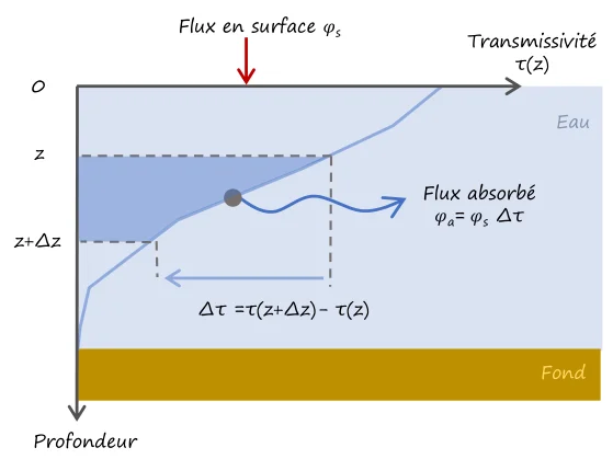
Let us now look at the flux absorbed by a slice of water at depth $z$, as presented below. The absorbed flux is given by the variation of the transmissivity with depth. The transmissivity decreases as a result of the absorption of radiation by its surrounding environment. We can therefore write that the absorbed flux in a slice between $z$ and $z +\Delta z$ is as:

$$ \varphi_{\text{a}} = -\left( \tau \left( z +\Delta z \right) - \tau(z) \right) \varphi_{\text{s}} $$

Absorption solaire — *Fig. 12: Solar flux absorbed by a water layer.*

Experimental validation

[to be continued]