Sensitivity Analysis
Introduction
Some models are complex or have a large number of parameters. In these situations it is often difficult to determine a ranking of the most influential parameters and to estimate their possible interactions. Various methods exist to address this issue, we focus here on sensitivity analysis using Morris’ method.
For example, let’s look at the animated image below. It shows the effect of a thrust on a solid and the displacement \(F\) that results from this. In short, we observe the behaviour of the function \(F\), the displacement, with respect to a parameter \(X\), the shape. We therefore obtain a variation \(\frac{\Delta F}{\Delta X}\), which is the quantity by which the observed function varied between two values of the parameter.
The idea of sensitivity analysis is to perform enough simulations to estimate the average effect of the variation of a parameter on the observed output.
Morris’ method principle
This method is known as a “One at a time” method, where only one parameter is changed at each simulation. The variation of the objective function \(F\) in relation to a parameter \(X_i\) is calculated by finite difference between two sets of identical parameters with the exception of a single parameter: see the figure below where the parameters are changed one by one and the so-called “elementary” effect of each is evaluated.
Thus, if there are \(d\) parameters, we need \(d+1\) simulations to assess the effect of a variation in each of them, i.e. \(\frac{\Delta F}{\Delta X_1},\frac{\Delta F}{\Delta X_2},…,\frac{\Delta F}{\Delta X_d}\).
In order to calculate an average elementary effect \(\frac{\Delta F}{\Delta X_i}\), we create \(d+1\) parameter sets and repeat the operation a \(r\) times. These are called “repetitions”.
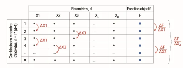
In total, we will therefore have achieved \(n=r\times(d+1)\) simulations. A commonly accepted value in the literature is \(r \sim 10\) or a total number of evaluations in the order of \(n \sim 10 \times d\).
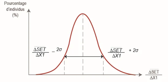
The series of elementary effects is then processed \(\frac{\Delta F}{\Delta X_i}\) of each parameter in order to calculate an average elementary effect \(\mu_i\) and a standard deviation \(\sigma_i\). For the record, more the standard deviation of a series is large, the more the values are scattered around the average. For example, the following figure represents the variation of an objective function with respect to parameter \(X_1\).
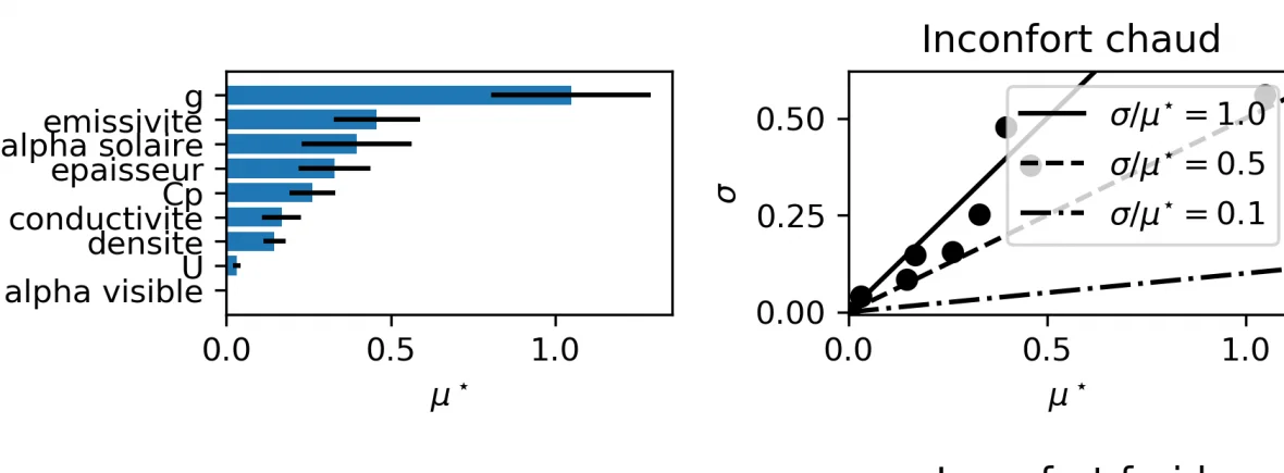
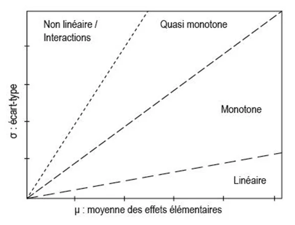
The classification of the parameters is then done according to the graph \((\mu,\sigma)\) as presented below. Influential parameters have a high average elementary effect: a variation in the parameter will result in a significant variation in the objective function. If the standard deviation of the series of elementary effects is small, the effect is considered linear. If this standard deviation is large, especially if it is of the order of magnitude of the elementary effect (i.e. greater than or equal to the first bisector), the effect is non-linear or causes interactions with other parameters.
Example
An example of a result applied to the building energy simulation of large volumes is given in this paragraph.
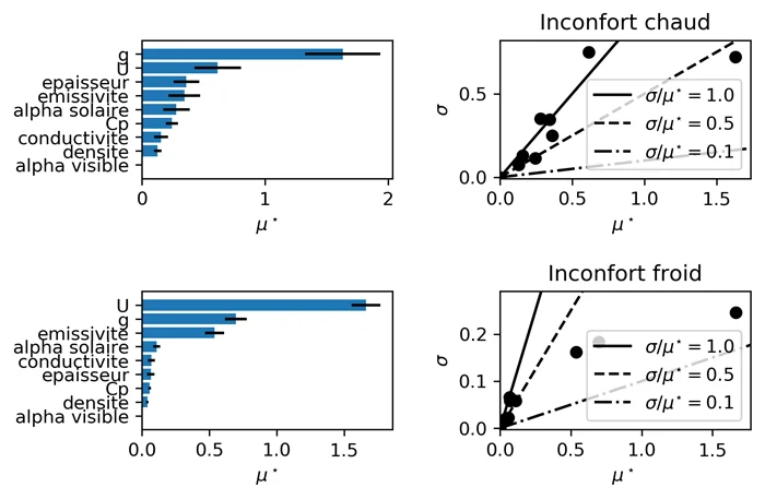
We want to know the most influential parameters when renovating a glazed canopy. The parameters chosen are the thickness, conductivity, mass heat capacity, density, solar & visible absorptivity and surface emissivity of the floor slab; the \(g\)-factor and \(U\)-factor of the glazing.
The objective function is the seasonal average of the differences between the SET index at time \(t\) and the center of the so-called comfortable SET range (i.e. the average of 22.2°C and 25.5°C SET). The winter and summer seasons are simulated: it can be seen that the classification of the parameters is not the same according to the season. The order of magnitude of the average elementary effect is \(\sim 1 [K]\) deviation from the comfort SET.
SAlibpython package link .