Genetic Optimization

The following content has been elaborated on the basis of the work done by G. Emperauger during his internship at AREP.

Introduction

Some problems in physics are irregular or not mathematically differentiable: an applied case for a building could be the choice between double and single glazing, or the open/closed position of a window. Classical resolution algorithms are inefficient in such cases because they are often based on the computation of a gradient to find solutions. In simple terms, classical methods look at the variation of a function with respect to an increment of the variable, however when the function is not continuous and therefore differentiable, it is difficult to calculate this gradient.

Genetic algorithms, imitating the natural selection of the most capable, propose an alternative solution to this problem that we will discuss here. The principle is to generate a set of potential solutions to the optimization problem (called “individuals”, and forming a “population”), and to make them evolve towards the optimal solution as the generations go by. Genetic algorithms are often confused with Particle Swarm Optimization (PSO) algorithms which work like a swarm of insects moving in space towards the best solution obtained by the swarm, without selecting the most suitable ones.

Principle

Darwinian selection of the fittest is based on the “survival” of individuals that are best adapted to their environment. The algorithm mimics this concept by selecting the combinations of parameters that are “fittest”, i.e. that minimize or maximize a cost function established by the user.

A genetic optimization procedure consists of the following steps (also shown in the figure below):

• The cross-breeding of individuals, mimicking chromosomal crossover, allows the exchange of characteristic traits of “parent” individuals to create the next generation.
• The application of stochastic mutations which bring a random component and allow to avoid staying on local minima, although they do not guarantee any result. When the mutation rate is important, the diversity of solutions is great but the algorithm can be slow to converge.
• The evaluation of the individuals with respect to the fixed objective of minimization/maximization: this is generally the time-consuming step of the calculation (in our applications it could be a dynamic thermal calculation).
• The ranking of individuals according to the chosen criteria.

Note that at the stage of evaluation of the individuals in the population, each individual can be evaluated independently, which offers an interesting potential for computational parallelization.

Necessarily, the size of the population is a performance factor for the algorithm: the larger it is, he better the solution space is scanned. However, the computational cost increases with the population size because all individuals must be evaluated.

Multi-objective optimization

In many cases, optimisation involves conciliating two contradictory objectives. For example, minimising both the environmental impact of the building materials chosen and the total cost of a structure involves two contradictory objectives (low-carbon materials are often more expensive). So we often optimise one objective to the detriment of another. In order to rank them in relation to each other, we introduce the notion of domination: in the figure below, with regard to objectives 1 and 2, the individual represented by the blue dot dominates the solutions located in the top right-hand orner but is dominated by those in the bottom left-hand corner. For the other two corners, the analysis is less straightforward because the blue dot is better for one objective and worse for the other.

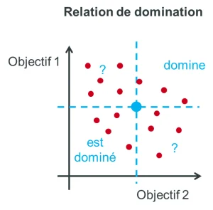
The set of solutions that are not dominated constitutes the Pareto front : On the type of graph such as the previous one, it is the low boundary of the cloud. In practice, these are the solutions for which we cannot improve one objective without degrading the secon

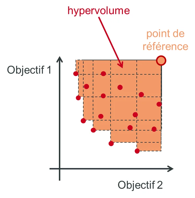
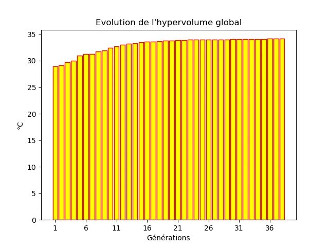
To evaluate the disparity of the solutions or the extent of the Pareto front, we introduce the notion of hypervolume. We place ourselves at the level of a reference point which is dominated by the set of solutions (see figure below) to be able to calculate the area between this point and the set of Pareto points. Numerically, dedicated libraries in different languages allow to compute it ( pygmo / pagmo ).

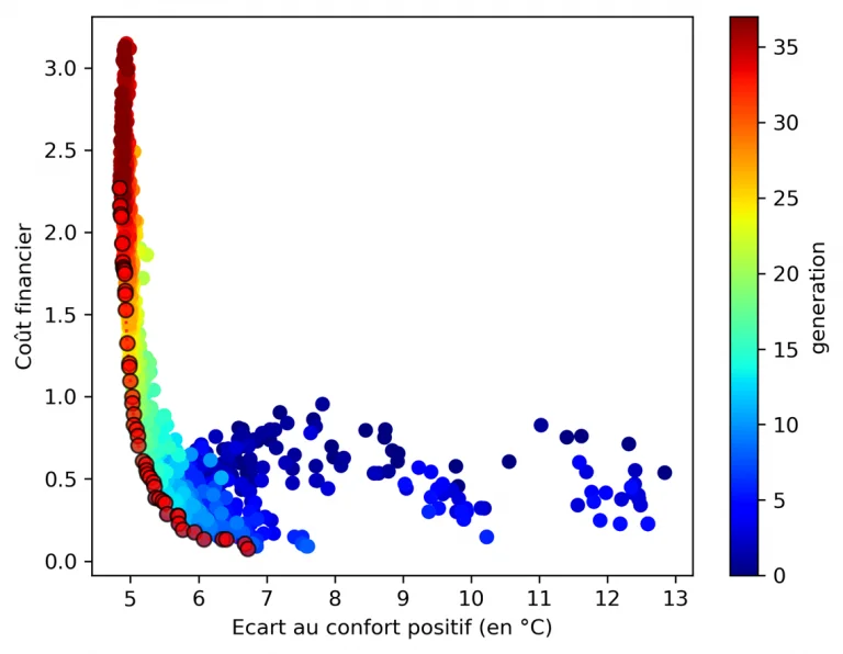
The hypervolume is also an indication of the convergence of the algorithm. Its evolution over the generations can give an idea of the convergence of the solutions, as shown on the example of the following figure.

Application examples

In this section we present some practical use cases.

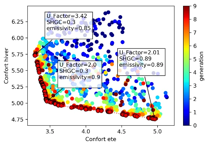
A use case of the method has been to determine for a glazed hall the combination between solar factor, thermal conductance \(U\) of the glazing and surface emissivity of the slab under the glass roof, in order to minimize the discomfort in summer and in winter. The result obtained is shown in the following figure. It can be seen that in winter high solar factors and low \(U\) coefficients dominate, while the opposite is true in summer.

A case of discrete optimization is the choice of the number and positioning of windows on a glazed facade, illustrated below (the aim is to maximize comfort in summer and reduce the cost of installing/maintaining windows - number and height - this will be detailed in a futur conference paper). We can see that the Pareto front is less “smooth” due to the discrete variables influencing the objective functions.

However, the choice of objective functions is crucial: they act as the algorithm’s “compass”. Thus when an objective function is badly chosen. As an example, the result below is a variant of the previous one: it consists in determining the position of a given number of windows on the studied façade. The objective function for cost was chosen such that it favors windows placed in height and thus the algorithm converged to this type of solution.