Field Projections and Interpolations

Introducing the problem

A common pitfall when solving problems with multiple physics is that the use of several tools often results in the creation of different meshes (see figure below). In this case, the fields need to be “projected” onto a common grid, so that calculations can be carried out at the same point in space for the two quantities being calculated.

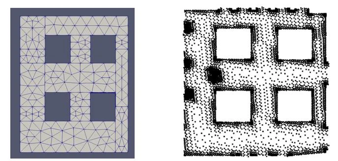
In the following section, a mathematical tool is presented to project one field onto another, regular or not.

Interpolation methods

There are several algorithms of varying complexity for producing a field projection. A few variations are presented in this section.

Nearest neighbors

One technique for projecting a field onto another is to solve a minimization problem. The brief method is explained here given in Aster code documentation in dimension two for the algorithm of the closest neighbors.

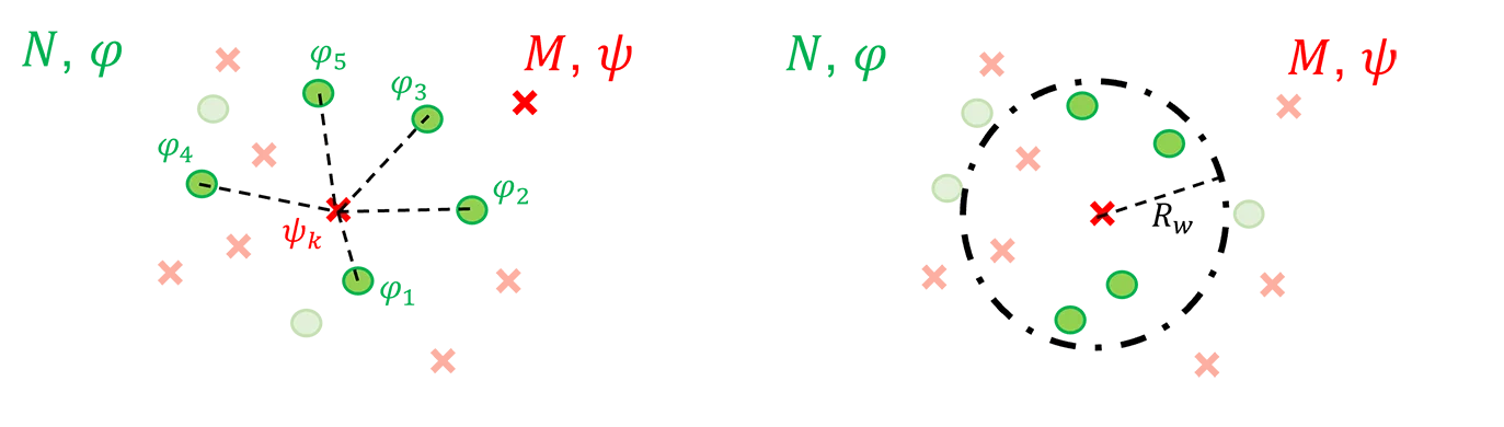
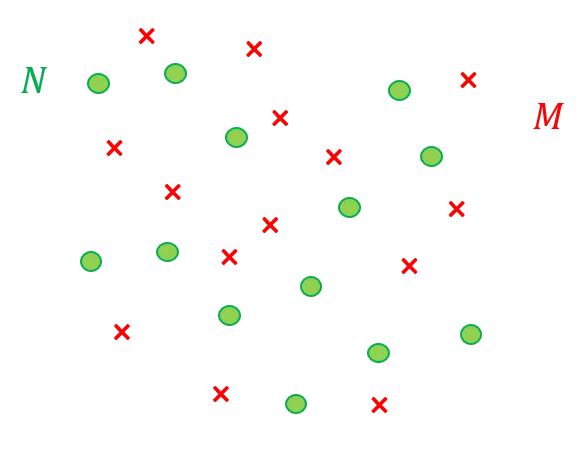
The aim is to project a cloud of points \(N\) bearing the field \(\varphi\) on a number of points \(M\) different of \(N\). Let us call \(\psi\) the projection of \(\varphi\) on \(M\).

Pour chaque point $k$ appartenant à $M$ de coordonnées $(x_k,y_k)$, on cherche ses $n$ plus proches voisins appartenant à $N$, ainsi qu’illustré sur la Figure qui suit. For each point \(k\) belonging \(M\) with coordinates \((x_k,y_k)\), we’re looking for its nnn nearest neighbors belonging to \(N\) as shown in following Figure.

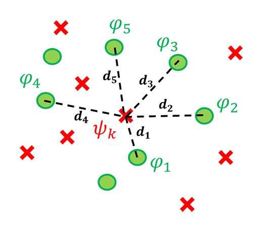
The value of the field on the projected point \(\psi_k\) is computed with coefficients \(a_k\), \(b_k\) and \(c_k\) such that:

$$ \psi_k = a_k + b_k x_k + c_k y_k $$

It is therefore a question of finding, for all points \(k\) of the cloud \(M\) the arrays \([a_k]\), \([b_k]\) and \([c_k]\) of coefficients that minimize the distance between the projected field \(\psi\) field and the original field \(\varphi\). Thus, for all point \(k\) of the cloud \(M\) we try to minimize the least squares \(\varepsilon_k\) between the \(\psi_k\) field and the original field \(\varphi_i\) on the \(n\) nearest neighbours.

$$ \varepsilon_k = \sum_{i=1}^{n} w(d_i) \big(\psi_k-\varphi_i \big)^2 $$

Where the weighting function \(w(d_i)\) depends on distance \(d_i\) between point \((x_i,y_i)\) of the initial cloud and point \(k\) of the projection grid \((x_k,y_k)\) :

$$ w(d_i) = \exp^{-(\frac{d_i}{d_{\text{r}}})^\beta} $$

Where:

• \(d_i\) is the distance between \((i-k)\) i.e. \(d_i=\sqrt{(x_i-x_k)^2+(y_i-y_k)^2}\),
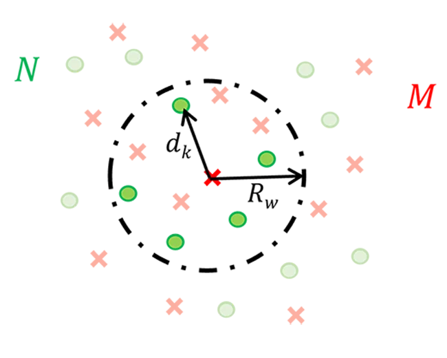
• \(d_{\text{r}}\) is the reference distance of the mesh. This is defined as the radius of the smallest circle centred at a point of \(M\) and containing three points of the cloud \(N\) as shown in the figure below (this radius can be determined with a kdtree from the scipy Python library for example). As a first approximation, if the distance \(\Delta_x\) between 2 points is known (e.g. in a regular mesh) we may consider \(d_{\text{r}} \sim \frac{\Delta x}{2}\). Otherwise, on can take the distance \(d_{\text{r}} \sim \frac{D^2}{N} = \frac{2D}{\sqrt{N}}\) where \(D\) is the greatest distance between any two points of the cloud.

The choice of the parameter set \((n,M,\beta,d_{\text{r}})\) will influence the global algorithm performance: given the cloud point distances one have to set a number \(M\) big enough, while keeping in mind that the calculation time is proportional to \(M\). Furthermore, chosing \(\beta>1\) implies that the nfluence of distant points is quickly soften when their distance from the reference point is greater than \(d_{\text{r}}\).

Tests conducted on analytical fields with a homogeneous point density have shown however that increasing the number of neighbors does not affect the quality of the projection. For such fields, the use of \(n \in [4,8]\) is recommended, with a weighting function coefficient of \(\beta=1.5\).

Shepard’s method

(adapted from T. Kliyam internship at AREP)

This method is a form of inverse distance weighting which is a spatial interpolation method. The main effort here will be to build an interpolation function \(Q(x,y)\) for the considered field, instead of using directly the value of the field.

In the analytical fields studied, this method is \(\sim \times 2\) more performant in terms of precision, for an execution time increasing by an order of magnitude. If the gain may seem small compared to the computation time, the robustness of Shepard’s method for the projection of real fields has been proven, in particular because it induces less smoothing on them.

Construction of an interpolation function on the initial field \(N\)

The simplest form of the method is called “Shepard’s method” (Shepard 1968¹), with the following equation:

$$ f\left(x,y\right)=\sum_{k=1}^{N}{w_k\left(x,y\right) F_k} $$

Where \(w_k\) is a weighting function generally dependent on distance and \(F_k\) is a function that calculates the value at the point \(k\). In the simplest cases, such as the nearest neighbor method, we define \(F_k=\varphi_k\) the value of the initial field at point \(k\).

In Shepard’s method, the weighting is defined as:

$$ w_k = \frac{\left[\frac{(R_k - d_k)_{+}}{R_k d_k}\right]^2}{\sum_{k=1}^{N}{\left[\frac{ (R_k-d_k)_{+} }{R_k d_k} \right]^2}} $$

Where:

• \(d_k\) is the distance between point \((x,y)\) and point \((x_k,y_k)\), i.e. \(d_k=\sqrt{\left(x-x_k\right)^2+\left(y-y_k\right)^2}\), with \(\left(x,y\right)\) the coordiantes of the interpolated point and \((x_k,y_k)\) the coordinates of the cloud of points of the initial field.
• \(R_{\text{q}}\) is the influence radius of a circle centered on the point \((x,y)\) represented on the figure below). In practice we choose \(N_{\text{q}} \sim 40 - 50\). The radius of influence is calculated so that:

$$ (R_{\text{q}} - d_k)_{+} = R_{\text{q}} - d_k \text{ for } d_k < R_{\text{q}} $$

$$ (R_{\text{q}}-d_k)_{+} = 0 \text{ for } d_k \ge R_{\text{q}} $$

Let \(D\) be the distance between the 2 most distant points of \(N\). We define \(R_{\text{q}}\) through the nodal function parameter \(N_{\text{q}}\) such that:

$$ R_{\text{q}}=\frac{D}{2}\sqrt{\frac{N_{\text{q}}}{N}} $$

As for the value of the function \(F_k\) we then construct an interpolation rule \(Q_k(x,y)\) defined as follows:

$$ Q_k(x,y)=\varphi_k+a_{k2}(x-x_k)+a_{k3}(y-y_k)+a_{k4}(x-x_k)^2 \\ +a_{k5}(x-x_k)(y-y_k)+a_{k6}(y-y_k)^2 $$

Where \(\varphi_k\) is the point value at \((x_k,y_k)\) and the coefficients \((a_{k2}, …,\ a_{k6})\) are specific to each point \((x_k,y_k)\). They are determined by the following least squares minimization, for \( k \in [1,N^\ast] \), where \( N^\ast \) is the number of points in the radius of influence \(R_{\text{q}}\) (for simplicity’s sake, the notations we will write indifferently \(N^\ast\) and \(N\) in the following, indeed, the weighting function cancels the contribution of the other points of the cloud):

$$ \varepsilon_k = \sum_{ i=1\ \text{and}\ i\neq k}^{N^*}\left [ \frac{Q_k(x_i,y_i)-\varphi_i}{\rho_k(x_i,y_i)} \right ]^2 $$

Explicitely:

$$ \varepsilon_k = \sum_{ i=1 \text{ and } i \neq k}^{N^*} \bigg [ \frac{(R_k - d_k)_{+}}{R_k d_k} \cdot \bigg ( \varphi_{k} + a_{k2}(x_i-x_k) + a_{k3}(y_i-y_k) + a_{k4}(x_i-x_k)^2 \\ + a_{k5}(x_i-x_k)(y_i-y_k) + a_{k6}(y_i-y_k)^2 - \varphi_i \bigg ) \bigg ]^2 $$

With \(d_i\) the distance between points \(i\) and \(k\) : \(d_i= \sqrt{(x_k-x_i)^2+(y_k-y_i)^2}\)

The interpolation equation then becomes:

$$ f(x,y)=\sum_{k=1}^{N^*}{w_k(x,y) \cdot Q_k(x,y)} $$

Note that the computational effort is located in the identification step of the parameters \(a_{2k},…, a_{6k}\): the greater the number \(N_{\text{q}}\) is, the larger the number of points involved, which increases the number of coefficients to be determined for the minimization function.

Calculation of the projection on the field \(M\)

We then define the radius of influence \(R_{\text{w}}\) of which an illustration is given in the Figure below, such that:

$$ R_{\text{w}}=\frac{D}{2}\cdot \sqrt{\frac{N_{\text{w}}}{N}} $$

In practice, an effective choice is to take \(N_{\text{w}}=N_{\text{q}}/2\).

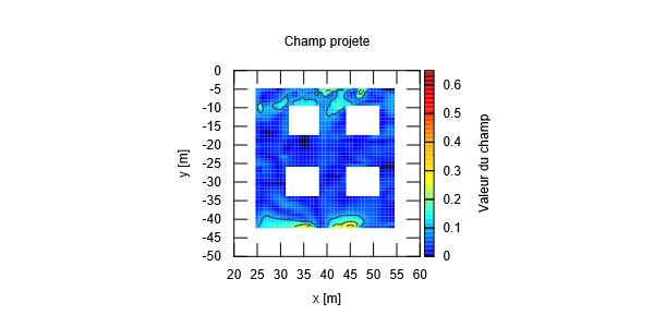
The projection on the point \((x_m,y_m)\) of the cloud \(M\) is calculated by summing the interpolation functions for each point in the radius of influence \(R_{\text{w}}\) (see figure below):

$$ \psi_m=\sum_{k=1}^{N}{w_k(x_m,y_m)}\cdot Q_k(x_m,y_m) $$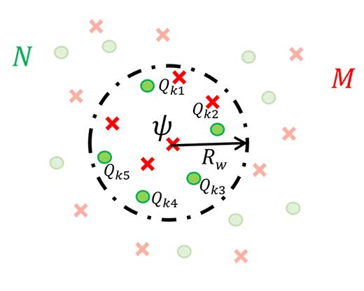

It is then necessary to calculate the projection \(\psi_m\) with the weighting function \(w_k\) defined analogously to the equation defined earlier whose radius of influence \(R_{\text{w}}\) is defined 2 equations earlier using the influence parameter \(N_{\text{w}}\).

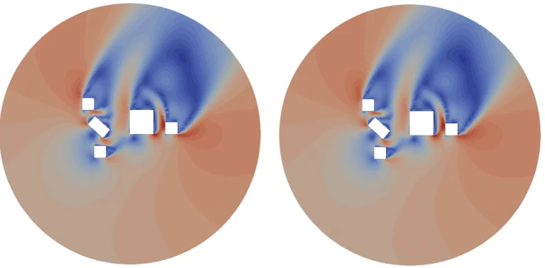
An applied example of Shepard’s method is shown below.

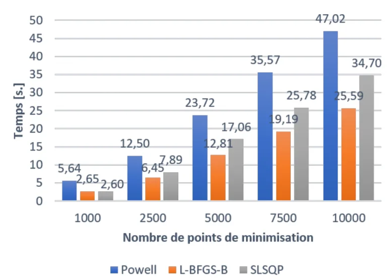
Results of the various minimisation algorithms on the execution time

Lastly, we try out some of the internal functions from the Optimize library from Scipy for an analytical 2D field projection problem. Interestingly, the L-BFGS-B method is the fastest. Above a threshold of about 2000 points on which we compute the interpollation function \(Q(x,y)\), one can notice a linear increase of the execution time.