Air Quality in subterranean train stations

Introduction & Starting point

Air quality in underground stations is a growing concern in cities with an urban transportation network. In France, continuous and open access measurement campaigns are carried out at the SNCF or at the RATP, giving access to data on the concentration of $PM_{2.5}$ and $PM_{10}$.

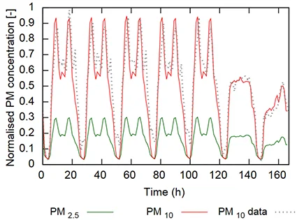
By using the available data, the correlation between rail traffic (continuous lines) and $PM_{10}$ (dotted line). The figure below represents an average week in the St-Michel Notre-Dame underground station (Paris). It can then be assumed that the majority of the amount of aerosol in suspension comes from braking and resuspension.

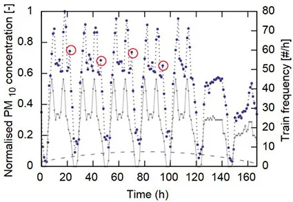
Corrélationconentration particules fines pm10 trafic ferroviaire — *Figure 1: Correlation between $PM_{10}$ concentration (grey solid line) and rail traffic (blue dotted lines)*

In this figure, it can be seen that the maximum $PM_{10}$ are concomitant with morning and evening traffic peaks, on the other hand, weekend concentrations decrease with rail traffic.

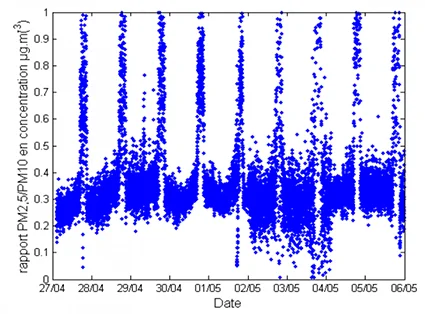
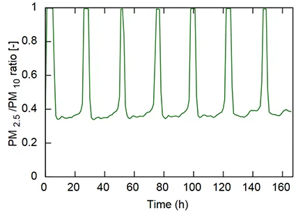
By observing the $PM_{2.5}/PM_{10}$ ration over one week at Magenta station (Paris) as shown in Figure 2 below from [Fortain, 2007] , we can see that it is between $\sim$ 0.2 and 0.35 during the day, while it reaches 1 during the night. The $PM_{2.5}$ being included in the $PM_{10}$, this means that the larger particles gradually disappear from the aerosol during the night time: only the finer ones remain.

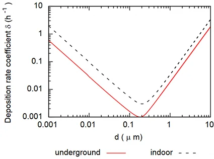
ratio pm2.5 pm10 gare particules fines — *Figure 2: Comparison between the $PM_{2.5}/PM_{10}$ ratio measured at Magenta from [Fortain 2007]*

This can be explained by the deposition rate of the particles. Indeed, it is more important for large diameter particles. Figure 3 below shows the deposition rate of particles as a function of their diameter based on [Lai et Nazaroff 2000] . Not surprisingly, gravity deposition is predominant for On particles larger than 1 [µm] in diameter. It should be noted that the finest particles, with a diameter of less than 0.01 [µm] also settle more significantly: this is related o the Brownian motion which diffuses very small particles onto surfaces. In the intermediate diameter range, the particles are too large to be subjected to the Brownian motion of the gas in which they evolve (air) and do not have enough mass for gravity sedimentation: the natural convection movements of the air are sufficient to keep them in suspension.

vitesse deposition diametre particules — *Figure 3: Deposition rate as a function of particle diameter.*

These observations have led to the development of successive models for predicting air quality in underground stations. The following sections describe the method developed in [Walther et Bogdan 2017a] and [Walther et al. 2017b] , available in the section Publications of this site.

Equations

Based on the previous finding and the homogeneous mixing hypothesis, a differential system is established that considers the concentrations of two classes of particles $C_{\text{a}}$ for the $PM_{2.5}$ and $C_{\text{b}}$ for the $PM_{2.5-10}$, the sum of the two being equal to the concentration of the $PM_{10}$. This makes it possible to capture the slower and faster ynamics of the aerosol particles:

$$ \frac{d C_{\text{a}}}{dt} = \alpha_{\text{a}} N^2(t) + \tau (C_{\text{a}}^\text{ext}-C_{\text{a}}) - \delta_{\text{a}} C_{\text{a}} $$

$$ \frac{d C_{\text{b}}}{dt} = \alpha_{\text{b}} N^2(t) + \tau (C_{\text{b}}^\text{ext}-C_{\text{b}}) - \delta_{\text{b}} C_{\text{b}} $$

Where $N$ is the number of trains per unit of time, $\alpha_{\text{a}}$, $\alpha_{\text{b}}$ are the terms of emission of the $PM_{2.5}$ and $PM_{2.5-10}$ and $\delta_{\text{a}},\delta_{\text{b}}$ he deposition rates calculated according to the [Lai et Nazaroff 2000] .

The air exchange rate $\tau$ is broken down into a natural ventilation rate $\tau_0$ and a piston effect ventilation $\beta \times N$, where $\beta$ [-] is the volume of utside air caused by the departure and the arrival of the train, divided by the volume of the station.

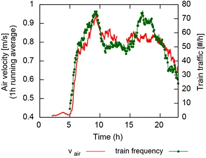
In the literature review by [Nicholson 1988]¹, the resuspension rate follows speed with a power law with an exponent ranging from 1 to 6. The apparent issue term $\alpha$ s thus assumed to vary with the square of the number of trains $N^2$: Indeed, if trains are iscrete events, they are considered to lead to an increase in the average speed at the station. The experimental air velocity measurement campaign conducted at St-Michel Notre-Dame station in February 2017 corroborates this hypothesis (see Figure 4 below).

vitesses d’air circulation train gare souterraine — *Figure 4: Measured air speed (sliding average over 1 hour) and train-traffic at St-Michel Notre-Dame station.*

Identification of model parameters

With the differential system in place, it remains to identify the unknown parameters of the model. There are six of them:

the piston effect $\beta$ whose order of magnitude can be determined by measurement or simulation (see our research on this subject),
the rate of air renewal by natural or mechanical ventilation $\tau_0$,
the apparent source terms $\alpha_{\text{a}}, \alpha_{\text{b}}$, which give the proportions of fine and larger particles emitted by braking and resuspension,
the deposition constants $\delta_{\text{a}}, \delta_{\text{b}}$ which are actually identified from equivalent aerosol diameters $d_{\text{a}},d_{\text{b}}$: indeed, the approach developed here considers that the total concentration of $PM_{10}$ is that of an aerosol composed of only two types of particles, in different concentrations.

The detailed identification of these parameters makes it possible to find fairly accurately the concentrations measured as a function of rail traffic, as shown in the Figure 5, where measurements and model are compared.

Comparaison modele mesure prediction concentration particules fines PM10 — *Figure 5: Model comparison (red) / measurement (dotted line).*

The $PM_{2.5}$ are also simulated by the model (see green curve in Figure 5) but without experimental confrontation, as these measurements are not available for the Saint-Michel station at the time of preparing this document (this paragraph will have to be updated).

The $PM_{2.5}/PM_{10}$ ratio obtained, presented in Figure 6, is very similar to the one of the experimental campaign of [Fortain, 2007] (see Figure 2).

ratio pm2.5 pm10 modele — *Figure 6: Simulated $PM_{2.5}/PM_{10}$ ratio*

Pending experimental results, this finding is considered to support the results obtained from the model. On this basis, it is possible to simulate the evolution of the $PM_{10}$ concentration as a function of ventilation and filtration installation, by integrating these terms into he model with the identified parameters.

Further development

The model is being improved, depending on the availability of measured data. Two major axes are being explored: the addition of the quantity deposited on surfaces and the generalization of a model to $n$ classes.

Closing equation

The addition of the equation on the surfaces closes the differential system previously presented as in [Qian et al. 2008] . This results in:

$$ V \times \frac{\partial C}{\partial t} = a N + Q_{\text{v}} (C^{\text{ext}} - C) - \delta V C + \rho S_{\text{r}}L $$

$$ S_{\text{d}} \times \frac{dL}{dt} = \delta V C - \rho S_{\text{r}} L $$

In the first equation, $V$ is the volume of the station, $Q_{\text{v}}$ is the external air flow rate, $\delta$ is the deposition rate, $\rho$ is the resuspension constant, $S_{\text{r}}$ the surface ccessible for resuspension and $L$ the quantity of particles deposited per unit area [µg/m²]. In the second equation, $S_{\text{d}}$ is the surface accessible for deposition.

It should be noted that these two equations are coupled by the cross terms $\pm \delta V C$ and $\pm \rho S_{\text{r}} L$. These respectively represent the quantity of particles that passes from the air “compartment” to the surface “compartment” by deposition and the quantity resuspended from the surfaces to the air volume.

Model with n classes

With a reasoning similar to that used for two particle size classes, it is possible to extend the model to $n$ classes: this would represent the evolution of an aerosol by size class, as shown in the following figure.

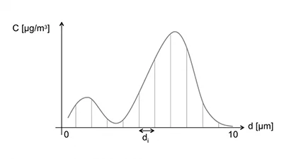
aerosol n classes tailles — *Schematic representation of an aerosol divided into n classes of particles.*

It becomes possible to define sources from their “emission spectrum” by size class. An example is given below:

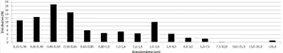
repratition granulometrique pm emission — *Example of granulometric distribution of an emission source.*

Among the scientific locks to be removed are the quantity of particles initially deposited, the differentiation of the resuspension term by size class (in other words: the “resuspension spectrum” for which there is not yet a unified theory) and finally the experimental comparison: external concentrations by size class are rarely available and the quantity of particles deposited on surfaces is difficult to evaluate.

Nicholson, K. W. (1988). A review of particle resuspension. Atmospheric Environment, 22(12), 2639-2651. DOI ↩︎